Model Development Variable Screening Variable Screening AKA Dimension

Model Development – Variable Screening

Variable Screening – AKA Dimension Reduction A more or less universally accepted principle: Principle of Parsimony

Variable screening – Univariate examination of candidate main effects.

A quick look at where we are – chd 2018_a

proc contents data=a. chd 2018_a position; run;

proc freq data=a. chd 2018_a nlevels; tables age--currsmok/noprint; run;

Continuous Target Categorical All categorical variables are coded 0, 1

t-tests /*a quick screen -- ttests*/ %let target=chd; %let continuous=age pulse chol hematocrit fvcht sbp bmi; %let categorical=diab male mi_chol mi_hem currsmok; ods select ttests; proc ttest data=a. chd 2018_a nobyvar plots=none; class ⌖ var &continuous &categorical; run;

Correlation

Pearson – detects linearity

Spearman – Pearson correlation of ranks. Less sensitive to nonlinearities and outliers than the Pearson

Hoeffding’s D detects a wide variety of associations between two variables.

/* another quick screen*/ %let target=chd; %let continuous=age pulse chol hematocrit fvcht sbp bmi; %let categorical=diab male mi_chol mi_hem currsmok; proc corr data=a. chd 2018_a spearman hoeffding; var ⌖ with &continuous &categorical; run;

Univariate logistics

/* another quick screen univariate models (partial)*/ %clearall ods select parameterestimates; proc logistic data=a. chd 2018_a descending; model chd=age; run; ods select parameterestimates; proc logistic data=a. chd 2018_a descending; model chd=pulse; run; ods select parameterestimates; proc logistic data=a. chd 2018_a descending; model chd=chol; run; ods select parameterestimates; proc logistic data=a. chd 2018_a descending; model chd=hematocrit; run;

%macro all_univ_betas(data=, depvar=, event=, indepvars=); %let numvars=%sysfunc(countw(&indepvars)); %put "Number of variables: " &numvars; %do i=1 %to &numvars; %let univ=%scan(&indepvars, &i); /*get ith variable*/ proc logistic data=&data; ods select parameterestimates; model &depvar(event="&event")=&univ; run; %end; %mend;

%clearall %let target=chd; %let continuous=age pulse chol hematocrit fvcht sbp bmi; %let categorical=diab male mi_chol mi_hem currsmok; options mprint; %all_univ_betas(data=a. chd 2018_a, depvar=chd, event=1, indepvars=&continuous &categorical) options nomprint;

Logit Plots(? )

A simple macro %macro all_logit_plots(data=, depvar=, indepvars=); %let numvars=%sysfunc(countw(&indepvars)); %put "Number of variables: " &numvars; %do i=1 %to &numvars; %let univ=%scan(&indepvars, &i); /*get ith variable*/ %Plot. Logits(indata=&data, numgrp=10, indepvar=&univ, depvar=&depvar); %end; %mend;

%clearall %let target=chd; %let continuous=age pulse chol hematocrit fvcht sbp bmi; %let categorical=diab male mi_chol mi_hem currsmok; options mprint; %all_logit_plots(data=a. chd 2018_a, depvar=chd, indepvars=&continuous); options nomprint;

A note on smoothers.

proc loess data=a. chd 2018_a; model chd=bmi/smooth=. 25. 5. 75 1 1. 25 1. 5; output out=smoothed predicted=phat; run; proc sort data=smoothed; by smoothingparameter bmi; run; data smoothed; set smoothed; where 0<phat<1; logit=log(phat/(1 -phat)); proc sgplot data=smoothed; series x=bmi y=logit/group=smoothingparameter lineattrs=(thickness=3); run;

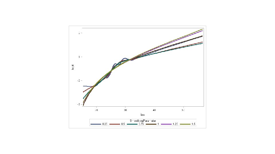
proc loess data=a. chd 2018_a; where bmi between 20 and 32; model chd=bmi/smooth=. 25. 5. 75 1 1. 25 1. 5; output out=smoothed predicted=phat; run; proc sort data=smoothed; by smoothingparameter bmi; run; data smoothed; set smoothed; where 0<phat<1; logit=log(phat/(1 -phat)); proc sgplot data=smoothed; series x=bmi y=logit/group=smoothingparameter lineattrs=(thickness=3); run;

An easier to modify program. %clearall %let var=chol; proc loess data=a. chd 2018_a; model chd=&var/smooth=. 25. 5. 75 1 1. 25 1. 5; output out=smoothed predicted=phat; run; proc sort data=smoothed; by smoothingparameter &var; run; data smoothed; set smoothed; where 0<phat<1; logit=log(phat/(1 -phat)); proc sgplot data=smoothed; series x=&var y=logit/group=smoothingparameter lineattrs=(thickness=3); run;

%clearall %let var=fvcht; proc loess data=a. chd 2018_a; model chd=&var/smooth=. 25. 5. 75 1 1. 25 1. 5; output out=smoothed predicted=phat; run; proc sort data=smoothed; by smoothingparameter &var; run; data smoothed; set smoothed; where 0<phat<1; logit=log(phat/(1 -phat)); proc sgplot data=smoothed; series x=&var y=logit/group=smoothingparameter lineattrs=(thickness=3); run;

Variable Screening Variable Clustering 31

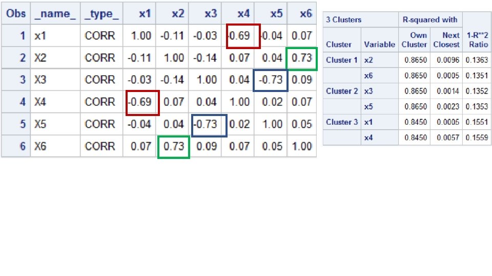
Variable Clustering Example title; data simpcorr (type=CORR); input _name_ $2. @4 _type_ $4. x 1 x 2 x 3 x 4 x 5 x 6; datalines; x 1 CORR 1 -. 11 -. 03 -. 69 -. 04. 07 X 2 CORR -. 11 1 -. 14. 07. 04. 73 X 3 CORR -. 03 -. 14 1. 04 -. 73. 09 X 4 CORR -. 69. 07. 04 1. 02. 07 X 5 CORR -. 04 -. 73. 02 1. 05 X 6 CORR. 07. 73. 09. 07. 05 1 ; run; proc contents data=simpcorr; run; proc print data=simpcorr; run;

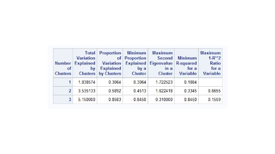
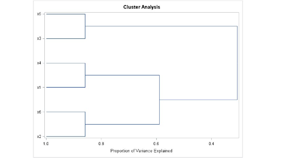
Variable Clustering Variable clustering finds groups of variables that are as correlated as possible among themselves and as uncorrelated as possible with variables in other clusters. The basic algorithm is binary and divisive. All variables start in one cluster. A principal components analysis is done on the variables in the cluster.

If the second eigenvalue is greater than a specified threshold (in other words, there is more than one dominant dimension), then the cluster is split. The PC scores are then rotated obliquely so that the variables can be split into two groups. This process is repeated for the two child clusters until the second eigenvalue drops below the threshold.

The VARCLUS Procedure PROC VARCLUS DATA=SAS-data-set <options>; VAR variables; RUN; proc varclus data=simpcorr; run; 37

data bodym; set nhanes 3. bodymeasurements (drop=BMPWTFLG BMPHTFLG); run; proc contents data=bodym position; run; proc corr data=bodym; var bm: ; run;

proc varclus data=bodym minclusters=3; var bm: ; run;

We formed clusters. What now? Pick one variable from each cluster. Principal components by cluster.