Model Checking A Brief Overview of the Algorithms

Model Checking A Brief Overview of the Algorithms Willem Visser Stellenbosch University

Overview • • • A Brief History of Model Checking My History of Model Checking The Models of Model Checking Temporal Logic Algorithms for Model Checking Retrospective With slides reused from a number of excellent researchers in the field: Ed Clarke, Randy Bryant, Ken Mc. Millan, Matt Dwyer, John Hatcliff and Tevfik Bultan

What is Model Checking • A form of Automated Finite State Verification – Does a finite state description of a system satisfy a behavioral property • If I press start, will the light eventually come on? – System description is a graph or transition relation – Property is specified in temporal logic • Is a system description a model for a temporal logic formula?

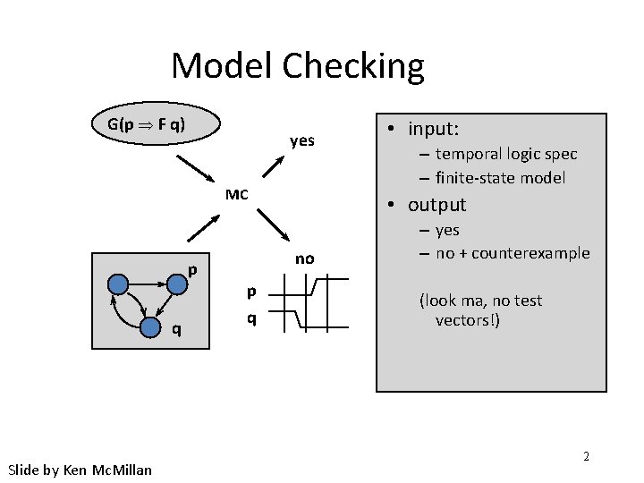
Model Checking G(p F q) yes MC p q Slide by Ken Mc. Millan – temporal logic spec – finite-state model • output no p q • input: – yes – no + counterexample (look ma, no test vectors!) 2

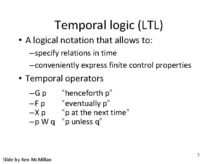
Temporal logic (LTL) • A logical notation that allows to: – specify relations in time – conveniently express finite control properties • Temporal operators –G p –F p –X p –p W q Slide by Ken Mc. Millan “henceforth p” “eventually p” “p at the next time” “p unless q” 5

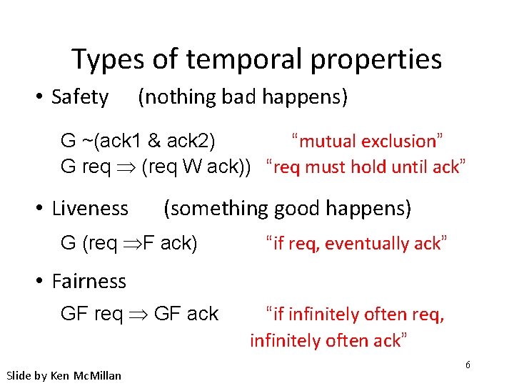
Types of temporal properties • Safety (nothing bad happens) G ~(ack 1 & ack 2) “mutual exclusion” G req (req W ack)) “req must hold until ack” • Liveness (something good happens) G (req F ack) “if req, eventually ack” • Fairness GF req GF ack Slide by Ken Mc. Millan “if infinitely often req, infinitely often ack” 6

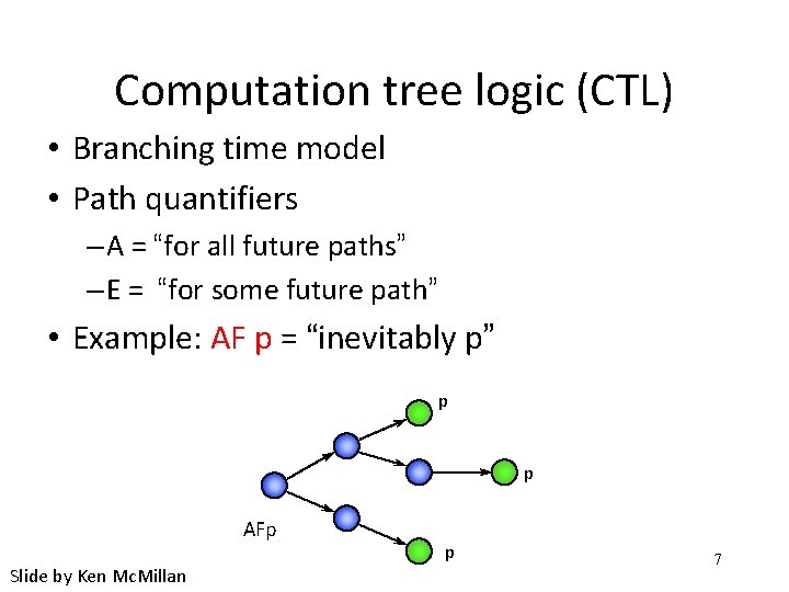
Computation tree logic (CTL) • Branching time model • Path quantifiers – A = “for all future paths” – E = “for some future path” • Example: AF p = “inevitably p” p p AFp Slide by Ken Mc. Millan p 7

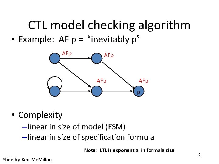
CTL model checking algorithm • Example: AF p = “inevitably p” AFp AFp p • Complexity – linear in size of model (FSM) – linear in size of specification formula Note: LTL is exponential in formula size Slide by Ken Mc. Millan 9

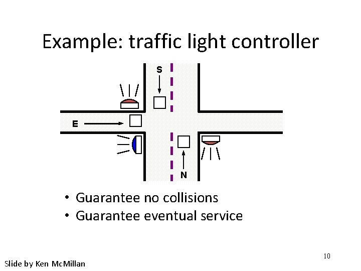
Example: traffic light controller S E N • Guarantee no collisions • Guarantee eventual service Slide by Ken Mc. Millan 10

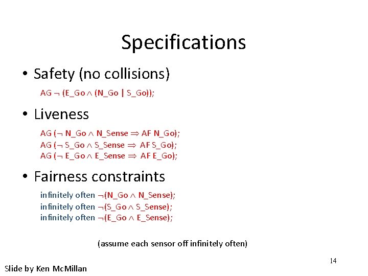
Specifications • Safety (no collisions) AG (E_Go (N_Go | S_Go)); • Liveness AG ( N_Go N_Sense AF N_Go); AG ( S_Go S_Sense AF S_Go); AG ( E_Go E_Sense AF E_Go); • Fairness constraints infinitely often (N_Go N_Sense); infinitely often (S_Go S_Sense); infinitely often (E_Go E_Sense); (assume each sensor off infinitely often) Slide by Ken Mc. Millan 14

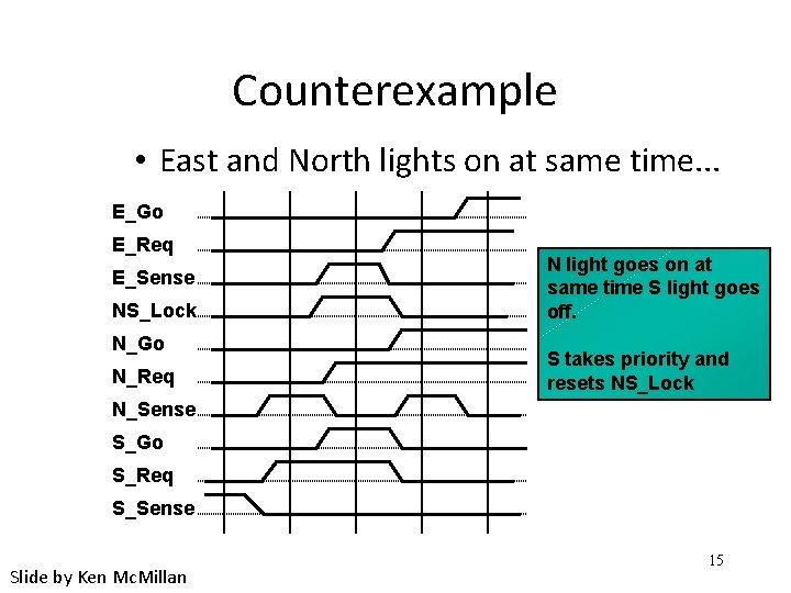
Counterexample • East and North lights on at same time. . . E_Go E_Req E_Sense NS_Lock N_Go N_Req N light goes on at same time S light goes off. S takes priority and resets NS_Lock N_Sense S_Go S_Req S_Sense Slide by Ken Mc. Millan 15

State explosion problem • What if the state space is too large? – too much parallelism – data in model • Approaches – Abstraction/reduction – “Symbolic” methods – Exploiting symmetry – “Partial order” methods Slide by Ken Mc. Millan 20

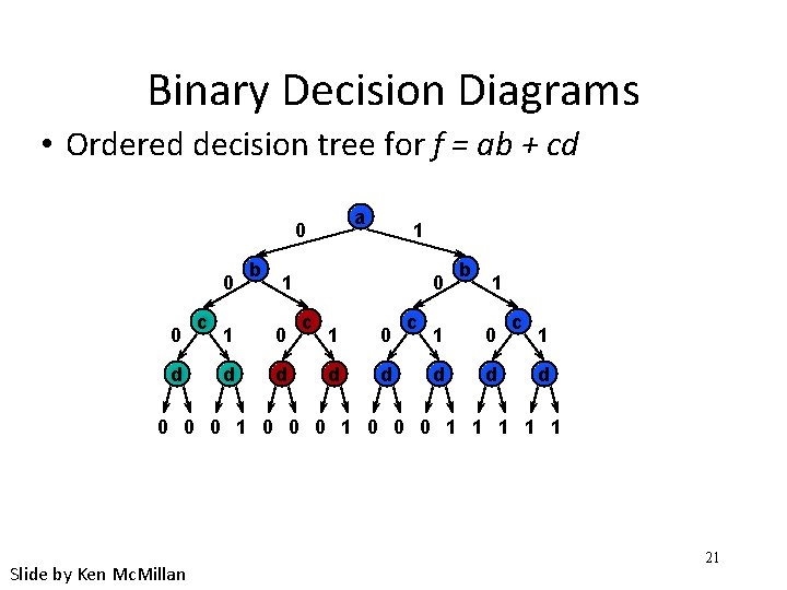
Binary Decision Diagrams • Ordered decision tree for f = ab + cd a 0 0 0 d c b 1 1 1 0 d d 0 c 1 0 d d c b 1 1 0 d d c 1 d 0 0 0 1 1 1 Slide by Ken Mc. Millan 21

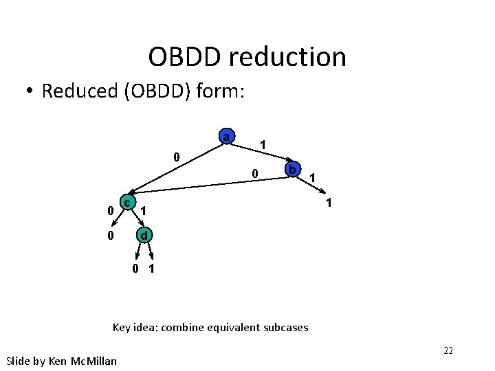
OBDD reduction • Reduced (OBDD) form: a 1 0 0 c b 1 1 1 d 0 1 Key idea: combine equivalent subcases Slide by Ken Mc. Millan 22

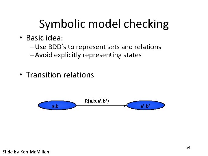
Symbolic model checking • Basic idea: – Use BDD’s to represent sets and relations – Avoid explicitly representing states • Transition relations a, b Slide by Ken Mc. Millan R(a, b, a’, b’) a’, b’ 24

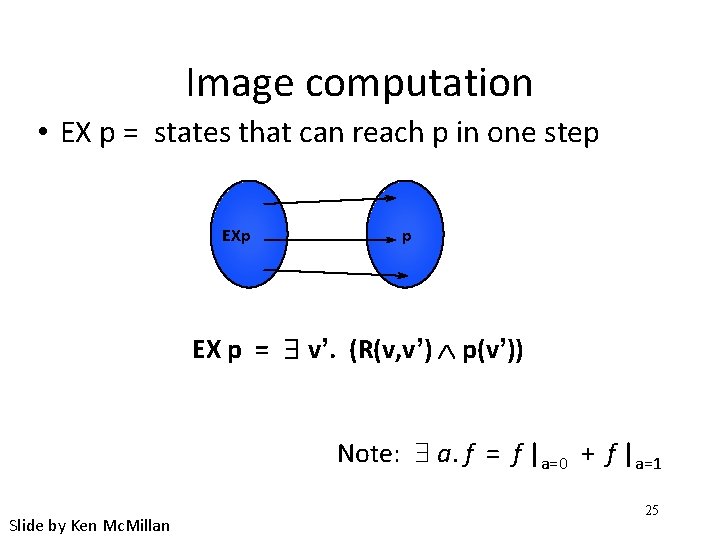
Image computation • EX p = states that can reach p in one step EXp p EX p = $ v’. (R(v, v’) Ù p(v’)) Note: a. f = f |a=0 + f |a=1 Slide by Ken Mc. Millan 25

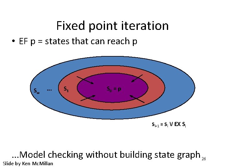
Fixed point iteration • EF p = states that can reach p Sw . . . S 1 S 0 = p Si+1 = Si / EX Si . . . Model checking without building state graph 26 Slide by Ken Mc. Millan

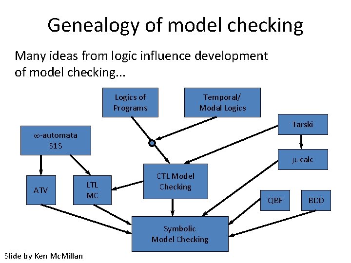
Genealogy of model checking Many ideas from logic influence development of model checking. . . Logics of Programs Temporal/ Modal Logics Tarski -automata S 1 S m-calc ATV LTL MC CTL Model Checking QBF Symbolic Model Checking Slide by Ken Mc. Millan BDD

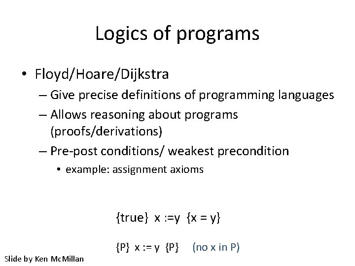
Logics of programs • Floyd/Hoare/Dijkstra – Give precise definitions of programming languages – Allows reasoning about programs (proofs/derivations) – Pre-post conditions/ weakest precondition • example: assignment axioms {true} x : =y {x = y} Slide by Ken Mc. Millan {P} x : = y {P} (no x in P)

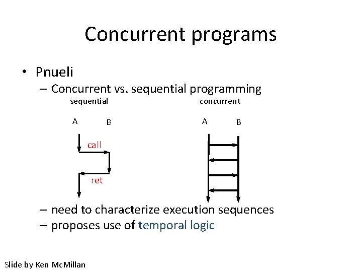
Concurrent programs • Pnueli – Concurrent vs. sequential programming sequential concurrent A A B B call ret – need to characterize execution sequences – proposes use of temporal logic Slide by Ken Mc. Millan

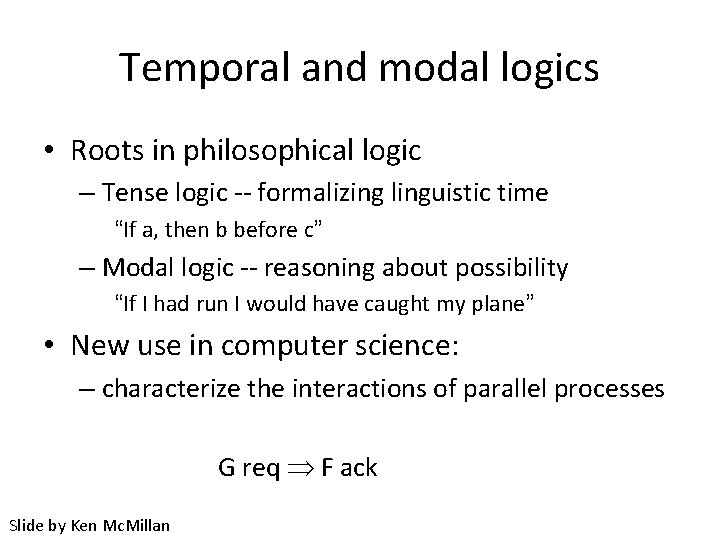
Temporal and modal logics • Roots in philosophical logic – Tense logic -- formalizing linguistic time “If a, then b before c” – Modal logic -- reasoning about possibility “If I had run I would have caught my plane” • New use in computer science: – characterize the interactions of parallel processes G req F ack Slide by Ken Mc. Millan

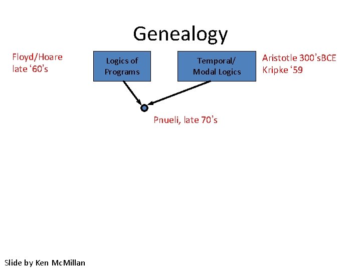
Genealogy Floyd/Hoare late ‘ 60’s Logics of Programs Temporal/ Modal Logics Pnueli, late 70’s Slide by Ken Mc. Millan Aristotle 300’s. BCE Kripke ‘ 59

CTL Model checking • Reasoning about properties of non-deterministic programs – branching time properties of programs – fixed point characterizations (Tarski) • every monotonic function has least/greatest fixed point – key idea: apply to finite graphs, not infinite trees • can directly calculate Tarski fixed points • Applications – finite state machines in hardware – protocols – proved incorrectness of some published designs Slide by Ken Mc. Millan

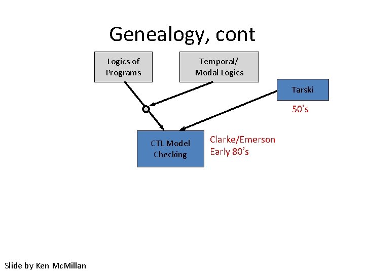
Genealogy, cont Logics of Programs Temporal/ Modal Logics Tarski 50’s CTL Model Checking Slide by Ken Mc. Millan Clarke/Emerson Early 80’s

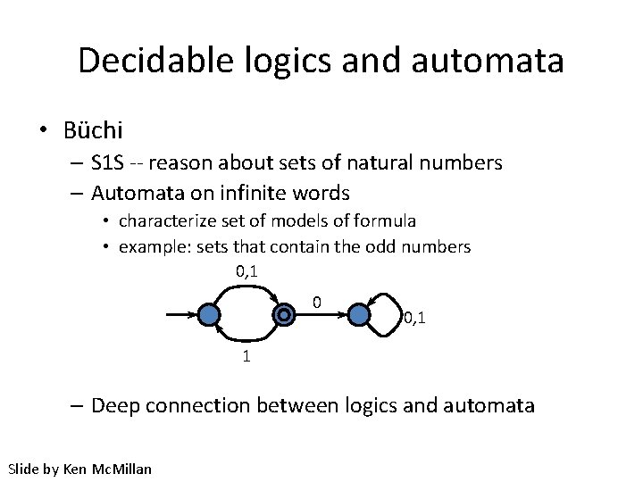
Decidable logics and automata • Büchi – S 1 S -- reason about sets of natural numbers – Automata on infinite words • characterize set of models of formula • example: sets that contain the odd numbers 0, 1 0 0, 1 1 – Deep connection between logics and automata Slide by Ken Mc. Millan

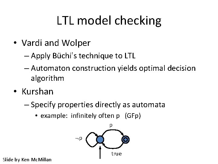
LTL model checking • Vardi and Wolper – Apply Büchi’s technique to LTL – Automaton construction yields optimal decision algorithm • Kurshan – Specify properties directly as automata • example: infinitely often p (GFp) p p Slide by Ken Mc. Millan true

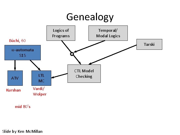
Genealogy Logics of Programs Büchi, 60 Temporal/ Modal Logics Tarski -automata S 1 S ATV Kurshan LTL MC Vardi/ Wolper mid 80’s Slide by Ken Mc. Millan CTL Model Checking

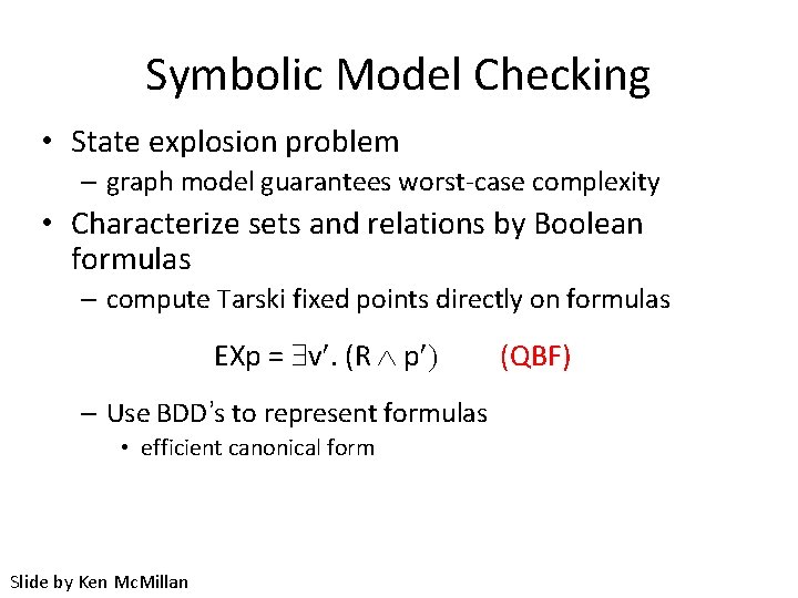
Symbolic Model Checking • State explosion problem – graph model guarantees worst-case complexity • Characterize sets and relations by Boolean formulas – compute Tarski fixed points directly on formulas EXp = v¢. (R p¢) (QBF) – Use BDD’s to represent formulas • efficient canonical form Slide by Ken Mc. Millan

Mu-calculus • Park’s Mu-Calculus – Logic of relations with fixed point operator – Can express transitive closure – Nicely characterizes what SMC can compute • SMC algorithm for Mu-calculus – Use to express symbolic algorithms for • CTL, LTL model checking AFp = m. Q. p AX Q • Automaton containment, etc. . . – Note: bad specification logic, but good for describing algorithms Slide by Ken Mc. Millan

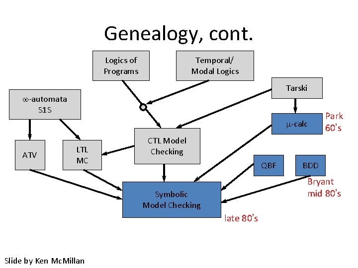
Genealogy, cont. Logics of Programs Temporal/ Modal Logics Tarski -automata S 1 S m-calc ATV LTL MC CTL Model Checking QBF BDD Bryant mid 80’s Symbolic Model Checking late 80’s Slide by Ken Mc. Millan Park 60’s

A convergence of research areas in logic • Many areas of logic have shaped the discourse in model checking – Logics of programs – Temporal/Modal logics – Tarski fixed point theory – Decidable logics -- S 1 S/automata – Park’s mu-calculus • Much of this work is quite abstract, but has strongly influenced practical work in model checking Slide by Ken Mc. Millan

Overview • • • A Brief History of Model Checking My History of Model Checking The Models of Model Checking Temporal Logic Algorithms for Model Checking Retrospective

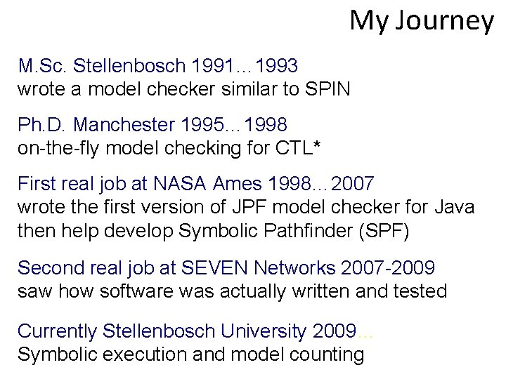
My Journey M. Sc. Stellenbosch 1991… 1993 wrote a model checker similar to SPIN Ph. D. Manchester 1995… 1998 on-the-fly model checking for CTL* First real job at NASA Ames 1998… 2007 wrote the first version of JPF model checker for Java then help develop Symbolic Pathfinder (SPF) Second real job at SEVEN Networks 2007 -2009 saw how software was actually written and tested Currently Stellenbosch University 2009… Symbolic execution and model counting

Models in Model Checking • Already know that “Model” Checking – Refers to the mathematical model for a temporal formula • There also other models – Often one refers to as what is being checked as a model – Finite state model checking requires a model of the environment to close the system • Hidden models – “Hidden models of model checking” • Visser, Dwyer, Whalen (2012) – Model checking is successful when intermediate models in the process is hidden from the user

Overview • • • A Brief History of Model Checking My History of Model Checking The Models of Model Checking Temporal Logic Algorithms for Model Checking Retrospective

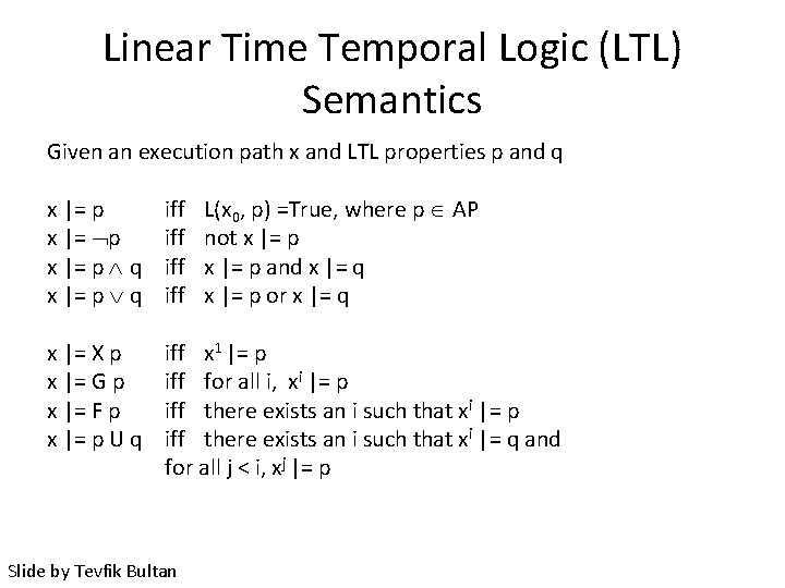
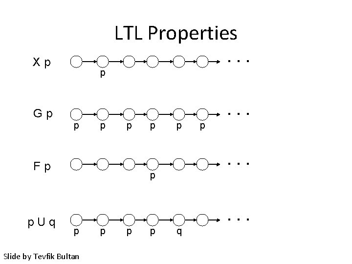
Linear Time Temporal Logic (LTL) Semantics Given an execution path x and LTL properties p and q L(x 0, p) =True, where p AP not x |= p and x |= q x |= p or x |= q x |= p q iff iff x |= X p x |= G p x |= F p x |= p U q iff x 1 |= p iff for all i, xi |= p iff there exists an i such that xi |= q and for all j < i, xj |= p Slide by Tevfik Bultan

LTL Properties Xp . . . p Gp p Fp p. Uq p p . . . p p Slide by Tevfik Bultan p p . . . q . . .

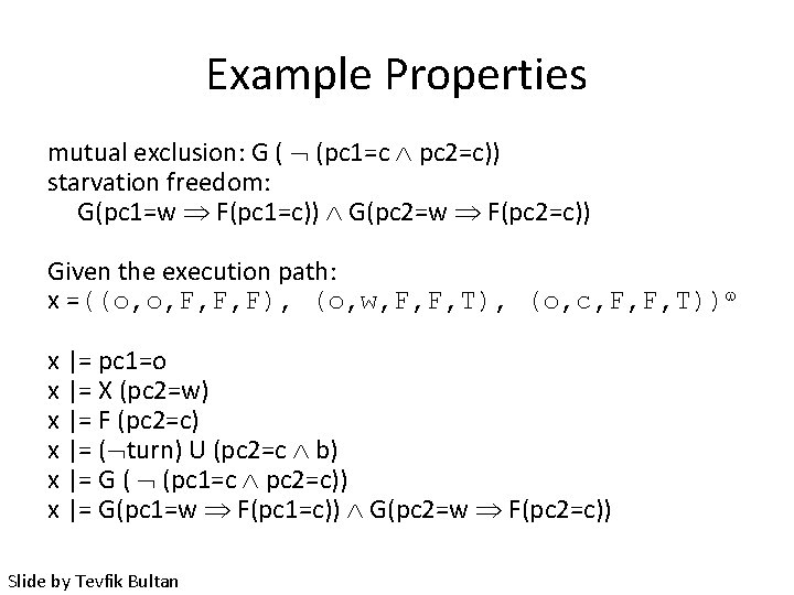
Example Properties mutual exclusion: G ( (pc 1=c pc 2=c)) starvation freedom: G(pc 1=w F(pc 1=c)) G(pc 2=w F(pc 2=c)) Given the execution path: x =((o, o, F, F, F), (o, w, F, F, T), (o, c, F, F, T)) x |= pc 1=o x |= X (pc 2=w) x |= F (pc 2=c) x |= ( turn) U (pc 2=c b) x |= G ( (pc 1=c pc 2=c)) x |= G(pc 1=w F(pc 1=c)) G(pc 2=w F(pc 2=c)) Slide by Tevfik Bultan

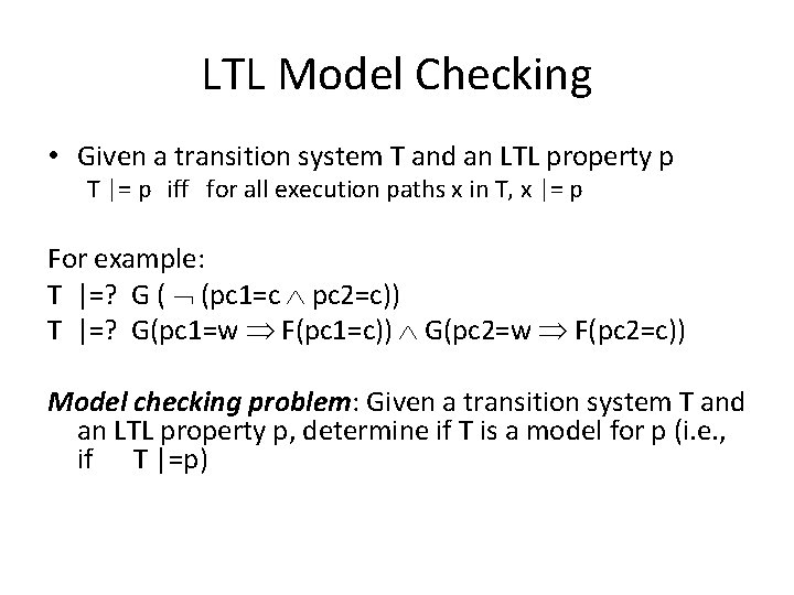
LTL Model Checking • Given a transition system T and an LTL property p T |= p iff for all execution paths x in T, x |= p For example: T |=? G ( (pc 1=c pc 2=c)) T |=? G(pc 1=w F(pc 1=c)) G(pc 2=w F(pc 2=c)) Model checking problem: Given a transition system T and an LTL property p, determine if T is a model for p (i. e. , if T |=p)

Linear Time vs. Branching Time • In linear time logics given we look at execution paths individually • In branching time logics we view the computation as a tree – computation tree: unroll the transition relation Transition System s 1 s 2 s 3 Execution Paths s 4 s 3. . . s 3 s 1 s 2 s 3. . . Slide by Tevfik Bultan Computation Tree s 4. . . s 4 s 1 s 3 s 2 s 3 s 1. . . s 4. . s 1. . .

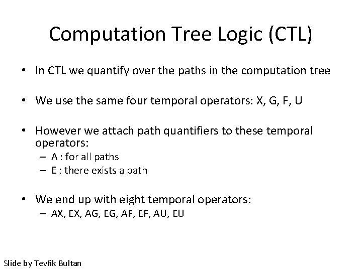
Computation Tree Logic (CTL) • In CTL we quantify over the paths in the computation tree • We use the same four temporal operators: X, G, F, U • However we attach path quantifiers to these temporal operators: – A : for all paths – E : there exists a path • We end up with eight temporal operators: – AX, EX, AG, EG, AF, EF, AU, EU Slide by Tevfik Bultan

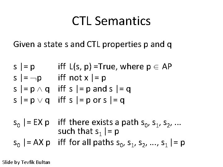
CTL Semantics Given a state s and CTL properties p and q s |= p q iff iff L(s, p) =True, where p AP not x |= p s |= p and s |= q s |= p or s |= q s 0 |= EX p iff there exists a path s 0, s 1, s 2, . . . such that s 1 |= p s 0 |= AX p iff for all paths s 0, s 1, s 2, . . . , s 1 |= p Slide by Tevfik Bultan

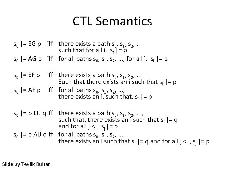
CTL Semantics s 0 |= EG p iff there exists a path s 0, s 1, s 2, . . . such that for all i, si |= p s 0 |= AG p iff for all paths s 0, s 1, s 2, . . . , for all i, si |= p s 0 |= EF p iff there exists a path s 0, s 1, s 2, . . . Such that there exists an i such that si |= p s 0 |= AF p iff for all paths s 0, s 1, s 2, . . . , there exists an i, such that, si |= p s 0 |= p EU q iff there exists a path s 0, s 1, s 2, . . . , such that, there exists an i such that si |= q and for all j < i, sj |= p s 0 |= p AU qiff for all paths s 0, s 1, s 2, . . . , there exists an I such that si |= q and for all j < i, sj |= p Slide by Tevfik Bultan

CTL Properties Transition System p s 1 s 2 s 3 |= p s 4 |= p s 1 |= p s 2 |= p Slide by Tevfik Bultan s 3 Computation Tree s 3 p p s 4 s 3 |= EX p s 3 |= EX p s 3 |= AX p s 3 |= EG p s 3 |= EG p s 3 |= AF p s 3 |= EF p s 3 |= AF p p s 4. . . s 4 p s 1 s 3 p s 2 s 3 p s 1. . . p s 4. . . s 1. . .

More Temporal Logics • CTL* – Superset of CTL and LTL • mu-Calculus – Even more expressive

Motivation Temporal properties are not always easy to write or read []((Q & !R & <>R) -> (P -> (!R U (S & !R))) U R) Hint: This a common structure that one would want to use in real systems Answer: P triggers S between Q (e. g. , end of system initialization) and R (start of system shutdown) Slides by Dwyer and Hatcliff

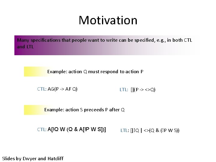
Motivation Many specifications that people want to write can be specified, e. g. , in both CTL and LTL Example: action Q must respond to action P CTL: AG(P -> AF Q) LTL: [](P -> <>Q) Example: action S preceeds P after Q CTL: A[!Q W (Q & A[!P W S])] Slides by Dwyer and Hatcliff LTL: []!Q | <>(Q & (!P W S))

Motivation We use Specification Patterns to… • Capture the experience base of expert designers • Transfer that experience between practioners • Classify properties – leverage in implementations • e. g. , specialize to a particular pattern of properties – allow informative communication about properties • e. g, “This is a response property with an after scope. ” Slides by Dwyer and Hatcliff

Other Classifications • Safety vs Liveness – Independent of a particular formalism • Practically, it is important to know the difference because… – It impacts how we design verification algorithms and tools • Some tools only check safety properties (e. g. , based on reachability algorithms) – It impacts how we run tools • Different command line options are used for Spin – It impacts how we form abstractions • Liveness properties often require forms of abstraction that differ from those used in safety properties Slides by Dwyer and Hatcliff

Safety Properties • Informally, a safety property states that nothing bad ever happens • Examples – Invariants: “x is always less than 10” – Deadlock freedom: “the system never reaches a state where no moves are possible” – Mutual exclusion: “the system never reaches a state where two processes are in the critical section” • As soon as you see the “bad thing”, you know the property is false • Safety properties can be falsified by a finite-prefix of an execution trace – Practically speaking, a Spin error trace for a safety property is a finite list of states beginning with the initial state Slides by Dwyer and Hatcliff

Liveness Properties • Informally, a liveness property states that something good will eventually happen • Examples – Termination: “the system eventually terminates” – Response properties: “if action X occurs then eventually action Y will occur” • Need to keep looking for the “good thing” forever • Liveness properties can be falsified by an infinite-suffix of an execution trace – Practically speaking, a Spin error trace for a liveness property is a finite list of states beginning with the initial state followed by a cycle showing you a loop that can cause you to get stuck and never reach the “good thing” Slides by Dwyer and Hatcliff

Assessment • Safety vs Liveness is an important distinction • However, it is very coarse – Lots of variations within safety and liveness – A finer classification might be more useful Slides by Dwyer and Hatcliff

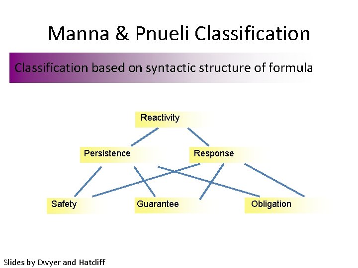
Manna & Pnueli Classification based on syntactic structure of formula Reactivity Persistence Safety Slides by Dwyer and Hatcliff Response Guarantee Obligation

Manna & Pnueli Classification Canonical Forms • • • Safety: [] p Guarantee: <> p Obligation: [] q || <> p Response: [] <> p Persistence: <> [] p Reactivite: []<>p || <>[]q Slides by Dwyer and Hatcliff

Assessment • The Manna-Pnueli classification is reasonable • However, their classification is based on the structure of formula, and we would like to avoid having engineers begin their reasoning by reasoning about the structure of formula • A classification based on the semantics of properties instead of syntax might be more useful for non-experts Slides by Dwyer and Hatcliff

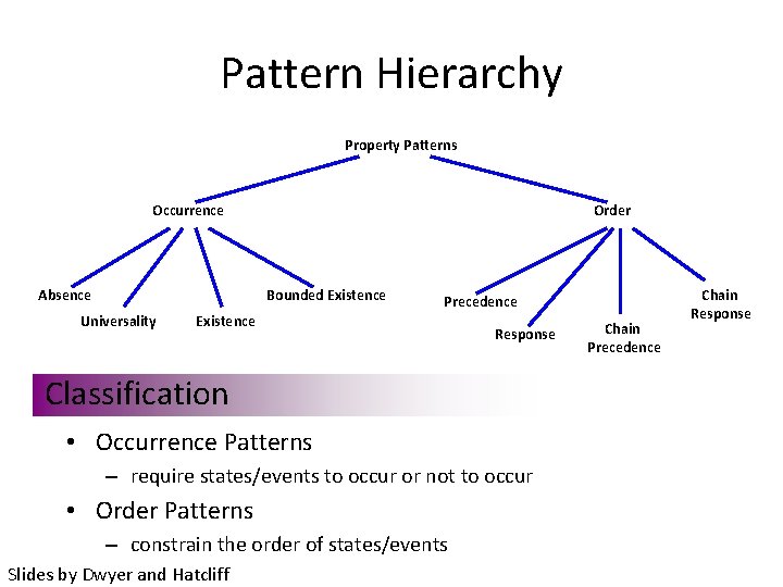
Pattern Hierarchy Property Patterns Occurrence Absence Order Bounded Existence Universality Precedence Existence Response Classification • Occurrence Patterns – require states/events to occur or not to occur • Order Patterns – constrain the order of states/events Slides by Dwyer and Hatcliff Chain Precedence Chain Response

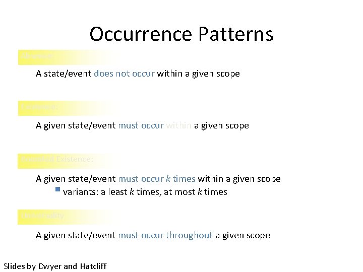
Occurrence Patterns Absence: A state/event does not occur within a given scope Existence: A given state/event must occur within a given scope Bounded Existence: A given state/event must occur k times within a given scope § variants: a least k times, at most k times Universality A given state/event must occur throughout a given scope Slides by Dwyer and Hatcliff

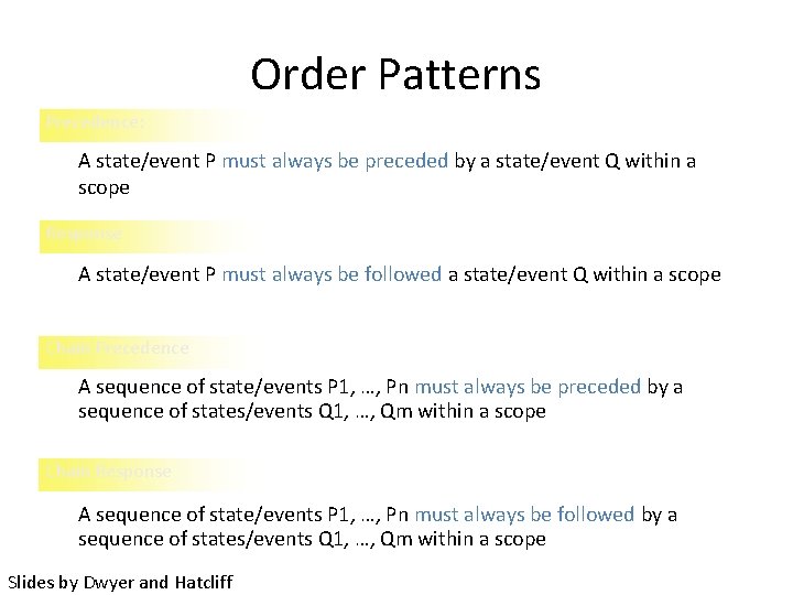
Order Patterns Precedence: A state/event P must always be preceded by a state/event Q within a scope Response A state/event P must always be followed a state/event Q within a scope Chain Precedence A sequence of state/events P 1, …, Pn must always be preceded by a sequence of states/events Q 1, …, Qm within a scope Chain Response A sequence of state/events P 1, …, Pn must always be followed by a sequence of states/events Q 1, …, Qm within a scope Slides by Dwyer and Hatcliff

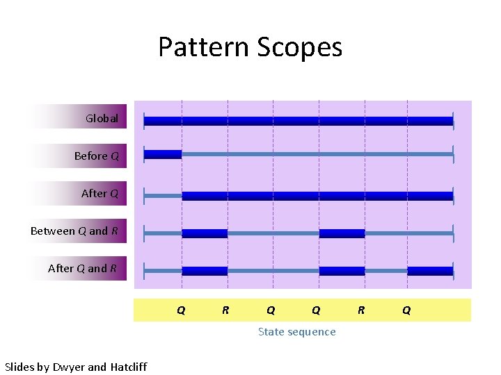
Pattern Scopes Global Before Q After Q Between Q and R After Q and R Q Q State sequence Slides by Dwyer and Hatcliff R Q

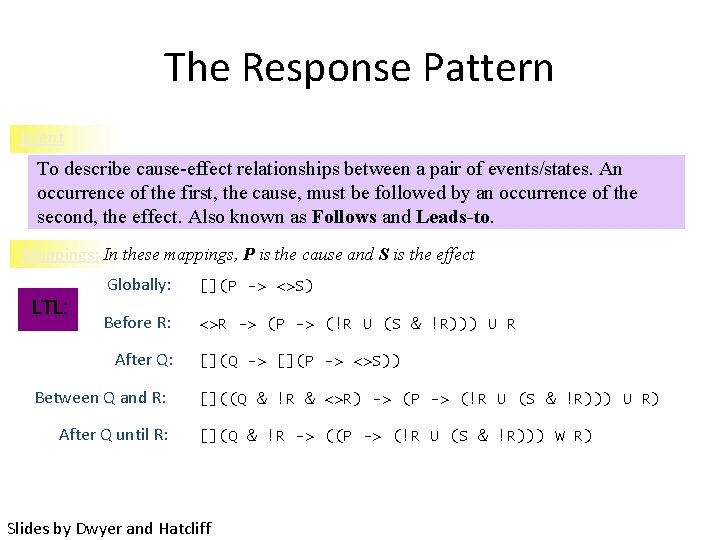
The Response Pattern Intent To describe cause-effect relationships between a pair of events/states. An occurrence of the first, the cause, must be followed by an occurrence of the second, the effect. Also known as Follows and Leads-to. Mappings: In these mappings, P is the cause and S is the effect LTL: Globally: [](P -> <>S) Before R: <>R -> (P -> (!R U (S & !R))) U R After Q: Between Q and R: After Q until R: [](Q -> [](P -> <>S)) []((Q & !R & <>R) -> (P -> (!R U (S & !R))) U R) [](Q & !R -> ((P -> (!R U (S & !R))) W R) Slides by Dwyer and Hatcliff

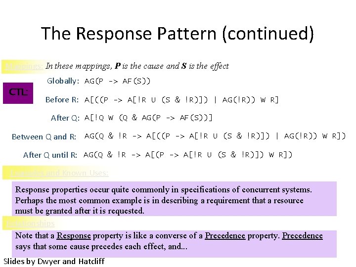
The Response Pattern (continued) Mappings: In these mappings, P is the cause and S is the effect CTL: Globally: AG(P -> AF(S)) Before R: A[((P -> A[!R U (S & !R)]) | AG(!R)) W R] After Q: A[!Q W (Q & AG(P -> AF(S))] Between Q and R: AG(Q & !R -> A[((P -> A[!R U (S & !R)]) | AG(!R)) W R]) After Q until R: AG(Q & !R -> A[(P -> A[!R U (S & !R)]) W R]) Examples and Known Uses: Response properties occur quite commonly in specifications of concurrent systems. Perhaps the most common example is in describing a requirement that a resource must be granted after it is requested. Relationships Note that a Response property is like a converse of a Precedence property. Precedence says that some cause precedes each effect, and. . . Slides by Dwyer and Hatcliff

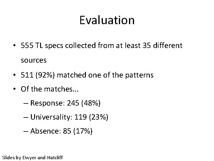
Evaluation • 555 TL specs collected from at least 35 different sources • 511 (92%) matched one of the patterns • Of the matches. . . – Response: 245 (48%) – Universality: 119 (23%) – Absence: 85 (17%) Slides by Dwyer and Hatcliff

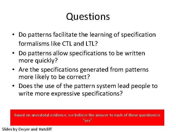
Questions • Do patterns facilitate the learning of specification formalisms like CTL and LTL? • Do patterns allow specifications to be written more quickly? • Are the specifications generated from patterns more likely to be correct? • Does the use of the pattern system lead people to write more expressive specifications? Based on anecdotal evidence, we believe the answer to each of these questions is “yes” Slides by Dwyer and Hatcliff

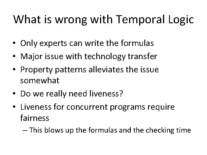
What is wrong with Temporal Logic • Only experts can write the formulas • Major issue with technology transfer • Property patterns alleviates the issue somewhat • Do we really need liveness? • Liveness for concurrent programs require fairness – This blows up the formulas and the checking time

Overview • • • A Brief History of Model Checking My History of Model Checking The Models of Model Checking Temporal Logic Algorithms for Model Checking Retrospective

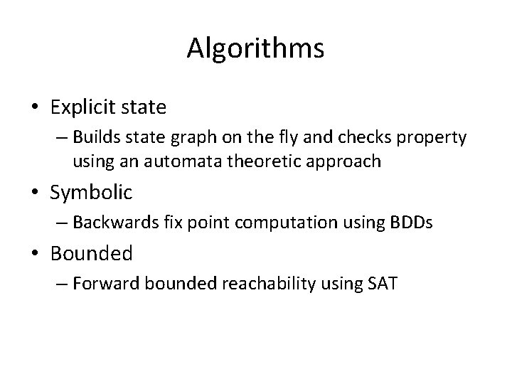
Algorithms • Explicit state – Builds state graph on the fly and checks property using an automata theoretic approach • Symbolic – Backwards fix point computation using BDDs • Bounded – Forward bounded reachability using SAT

Model Checking The Intuition • Calculate whether a system satisfies a certain behavioral property: – Is the system deadlock free? – Whenever a packet is sent will it eventually be received? • So it is like testing? No, major difference: – Look at all possible behaviors of a system • Automatic, if the system is finite-state – Potential for being a push-button technology – Almost no expert knowledge required • How do we describe the system? • How do we express the properties? 24 September 2002 © Willem Visser 2002 67

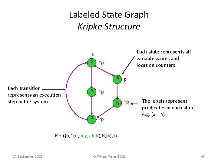
Labeled State Graph Kripke Structure Each state represents all variable values and location counters x ~p k p Each transition represents an execution step in the system y ~p hh ~p z ~p The labels represent predicates in each state e. g. (x = 5) K = ({p, ~p}, {x, y, z, k, h}, R, {x}, L) 24 September 2002 © Willem Visser 2002 68

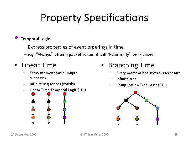
Property Specifications • Temporal Logic – Express properties of event orderings in time – e. g. “Always” when a packet is sent it will “Eventually” be received • Linear Time • Branching Time – Every moment has a unique successor – Infinite sequences (words) – Linear Time Temporal Logic (LTL) 24 September 2002 © Willem Visser 2002 – Every moment has several successors – Infinite tree – Computation Tree Logic (CTL) 69

Safety and Liveness • Safety properties – Invariants, deadlocks, reachability, etc. – Can be checked on finite traces – “something bad never happens” • Liveness Properties – Fairness, response, etc. – Infinite traces – “something good will eventually happen” 24 September 2002 © Willem Visser 2002 70

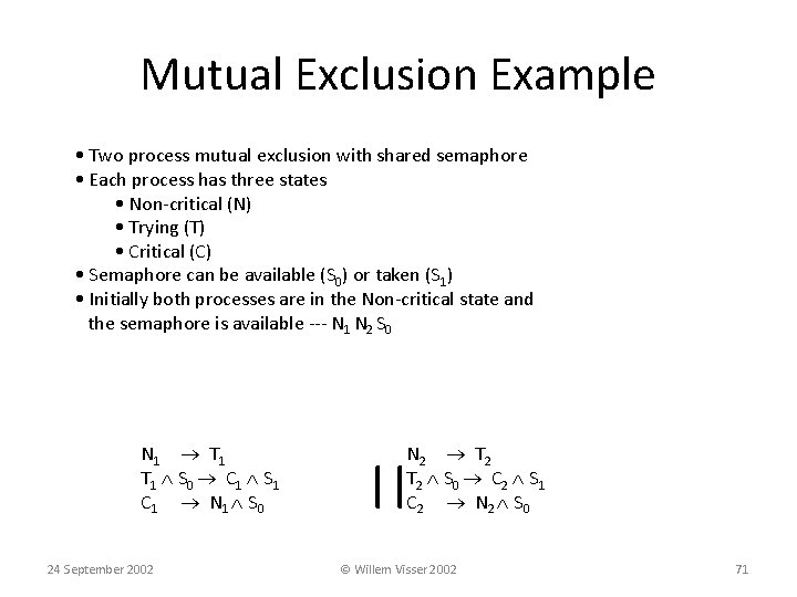
Mutual Exclusion Example • Two process mutual exclusion with shared semaphore • Each process has three states • Non-critical (N) • Trying (T) • Critical (C) • Semaphore can be available (S 0) or taken (S 1) • Initially both processes are in the Non-critical state and the semaphore is available --- N 1 N 2 S 0 N 1 T 1 S 0 C 1 S 1 C 1 N 1 S 0 24 September 2002 N 2 T 2 S 0 C 2 S 1 C 2 N 2 S 0 || © Willem Visser 2002 71

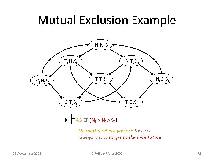
Mutual Exclusion Example N 1 N 2 S 0 T 1 N 2 S 0 N 1 T 2 S 0 T 1 T 2 S 0 C 1 N 2 S 1 C 1 T 2 S 1 N 1 C 2 S 1 T 1 C 2 S 1 K ╞ AG EF (N 1 N 2 S 0) No matter where you are there is always a way to get to the initial state 24 September 2002 © Willem Visser 2002 72

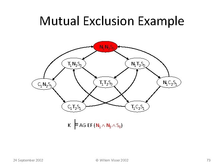
Mutual Exclusion Example N 1 N 2 S 0 T 1 N 2 S 0 N 1 T 2 S 0 T 1 T 2 S 0 C 1 N 2 S 1 C 1 T 2 S 1 N 1 C 2 S 1 T 1 C 2 S 1 K ╞ AG EF (N 1 N 2 S 0) 24 September 2002 © Willem Visser 2002 73

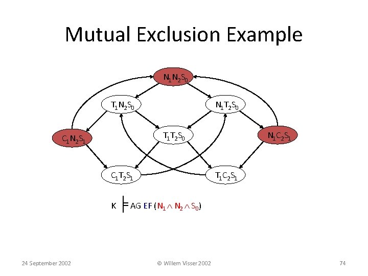
Mutual Exclusion Example N 1 N 2 S 0 T 1 N 2 S 0 N 1 T 2 S 0 T 1 T 2 S 0 C 1 N 2 S 1 C 1 T 2 S 1 N 1 C 2 S 1 T 1 C 2 S 1 K ╞ AG EF (N 1 N 2 S 0) 24 September 2002 © Willem Visser 2002 74

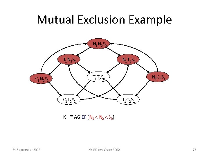
Mutual Exclusion Example N 1 N 2 S 0 T 1 N 2 S 0 N 1 T 2 S 0 T 1 T 2 S 0 C 1 N 2 S 1 C 1 T 2 S 1 N 1 C 2 S 1 T 1 C 2 S 1 K ╞ AG EF (N 1 N 2 S 0) 24 September 2002 © Willem Visser 2002 75

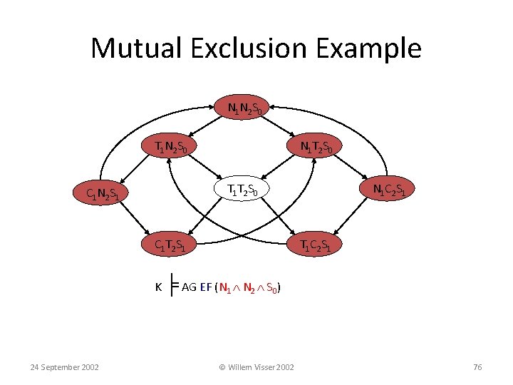
Mutual Exclusion Example N 1 N 2 S 0 T 1 N 2 S 0 N 1 T 2 S 0 T 1 T 2 S 0 C 1 N 2 S 1 C 1 T 2 S 1 N 1 C 2 S 1 T 1 C 2 S 1 K ╞ AG EF (N 1 N 2 S 0) 24 September 2002 © Willem Visser 2002 76

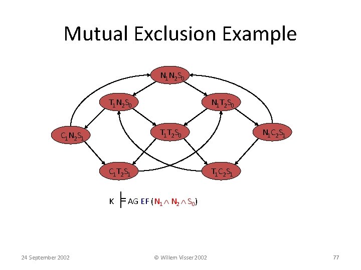
Mutual Exclusion Example N 1 N 2 S 0 T 1 N 2 S 0 N 1 T 2 S 0 T 1 T 2 S 0 C 1 N 2 S 1 C 1 T 2 S 1 N 1 C 2 S 1 T 1 C 2 S 1 K ╞ AG EF (N 1 N 2 S 0) 24 September 2002 © Willem Visser 2002 77

Model Checking • Given a Kripke structure M = (S, R, L) that represents a finite-state concurrent system and a temporal logic formula f expressing some desired specification, find the set of states in S that satisfy f: { s S | M, s ╞ f } • Normally, some states of the concurrent system are designated as initial states. The system satisfies the specification provided all the initial states are in the set. We often write: M ╞ f 24 September 2002 © Willem Visser 2002 78

Explicit State Model Checking • • • Typically Automata theoretic model checking Enumerates all system states Typically on-the-fly Exponential in the size of the formula Linear in the size of the system Many popular model checkers work this way – SPIN, Java Path. Finder

Automata-based LTL Model Checking • Büchi automata: Finite state automata that accept infinite strings – The better known variant of finite state automata accept finite strings (used in lexical analysis for example) • A Büchi automaton accepts a string when the corresponding run visits an accepting state infinitely often – Note that an infinite run never ends, so we cannot say that an accepting run ends at an accepting state • LTL properties can be translated to Büchi automata – The automaton accepts a path if and only if the path satisfies the corresponding LTL property Slide by Tevfik Bultan

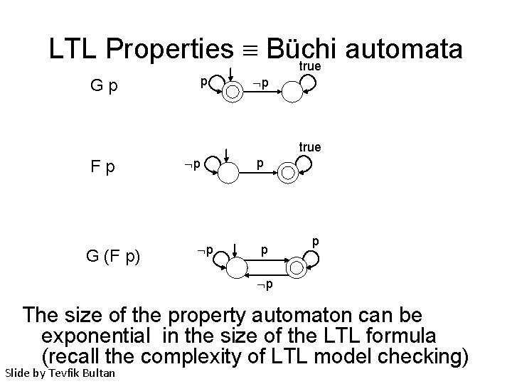
LTL Properties Büchi automata true Gp p p true Fp G (F p) p p The size of the property automaton can be exponential in the size of the LTL formula (recall the complexity of LTL model checking) Slide by Tevfik Bultan

Büchi Automata: Language Emptiness Check • Given a Buchi automaton, one interesting question is: – Is the language accepted by the automaton empty? • i. e. , does it accept any string? • A Büchi automaton accepts a string when the corresponding run visits an accepting state infinitely often • To check emptiness: – Look for a cycle which contains an accepting state and is reachable from the initial state • Find a strongly connected component that contains an accepting state, and is reachable from the initial state – If no such cycle can be found the language accepted by the automaton is empty Slide by Tevfik Bultan

LTL Model Checking • Generate the property automaton from the negated LTL property • Generate the product of the property automaton and the transition system • Show that there is no accepting cycle in the product automaton (check language emptiness) – i. e. , show that the intersection of the paths generated by the transition system and the paths accepted by the (negated) property automaton is empty • If there is a cycle, it corresponds to a counterexample behavior that demonstrates the bug Slide by Tevfik Bultan

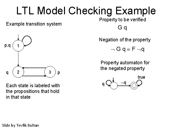
LTL Model Checking Example transition system Property to be verified Gq Negation of the property p, q q 1 2 G q F q 3 p Each state is labeled with the propositions that hold in that state Slide by Tevfik Bultan Property automaton for the negated property true q q

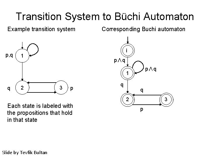
Transition System to Büchi Automaton Example transition system p, q Corresponding Buchi automaton i 1 p∧q 1 q 2 3 p q q 2 Each state is labeled with the propositions that hold in that state Slide by Tevfik Bultan 3 p

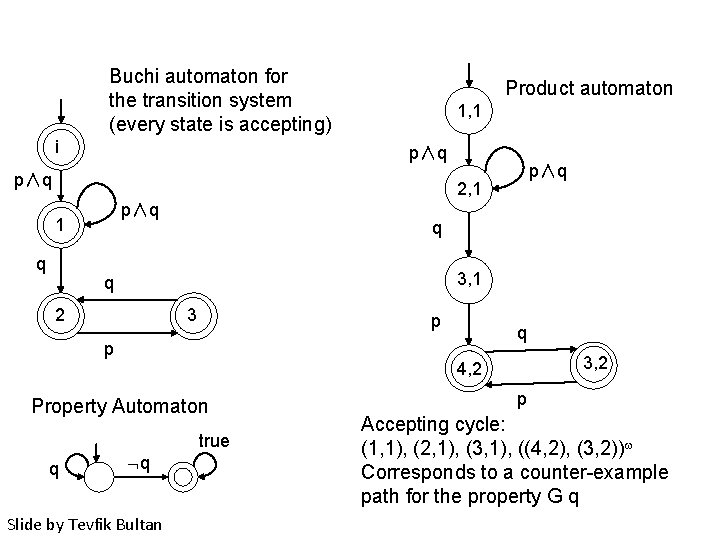
Buchi automaton for the transition system (every state is accepting) i Product automaton 1, 1 p∧q p∧q 2, 1 p∧q 1 q q 3, 1 q 2 3 p q p 3, 2 4, 2 Property Automaton true q q Slide by Tevfik Bultan p Accepting cycle: (1, 1), (2, 1), (3, 1), ((4, 2), (3, 2)) Corresponds to a counter-example path for the property G q

How to make things efficient • Nested DFS search for accepting cycles • Bitstate hashing to save memory

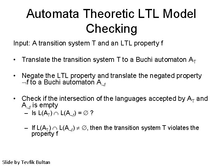
Automata Theoretic LTL Model Checking Input: A transition system T and an LTL property f • Translate the transition system T to a Buchi automaton AT • Negate the LTL property and translate the negated property f to a Buchi automaton A f • Check if the intersection of the languages accepted by AT and A f is empty – Is L(AT) L(A f) = ? – If L(AT) L(A f) , then the transition system T violates the property f Slide by Tevfik Bultan

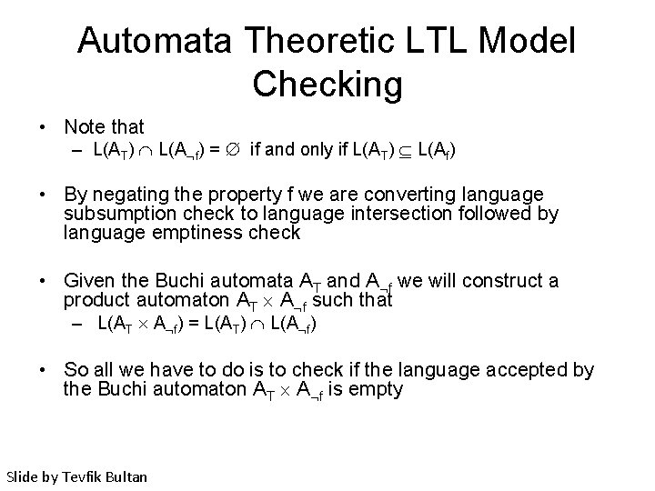
Automata Theoretic LTL Model Checking • Note that – L(AT) L(A f) = if and only if L(AT) L(Af) • By negating the property f we are converting language subsumption check to language intersection followed by language emptiness check • Given the Buchi automata AT and A f we will construct a product automaton AT A f such that – L(AT A f) = L(AT) L(A f) • So all we have to do is to check if the language accepted by the Buchi automaton AT A f is empty Slide by Tevfik Bultan

Finding Reachable Cycles • To find cycles in a graph one can use a depth-first search algorithm which constructs the strongly connected components in linear time by adding two integer numbers to every state reached [Tarjan, 72] • If a strongly connected component reachable from an initial state contains an accepting state then the language accepted by the Buchi automaton is not empty. • There is a more memory efficient algorithm for checking the same condition which is called nested depth first search. Slide by Tevfik Bultan

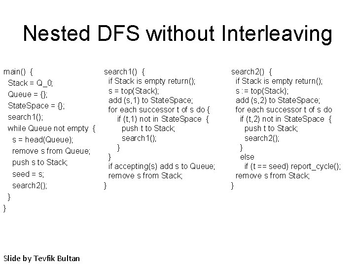
Nested Depth First Search [Corcoubetis, Vardi, Wolper, Yannakakis 92] • Do a depth first search from the initial states – While doing this search build a postorder list (children appear before their parents) of reachable accepting states. Let this ordered list be L = q 1, q 2, … , qk where q 1 is the first postorder reachable state and qk is the last. • Do a second depth first search from the elements in L – Start the search from q 1 – Once the search from qi is finished (either qi is reached, i. e. , a cycle is found, or there are no more reachable states from qi), restart the search from qi+1 but do not reconsider the states that have been visited during searches from qj, for j i. Slide by Tevfik Bultan

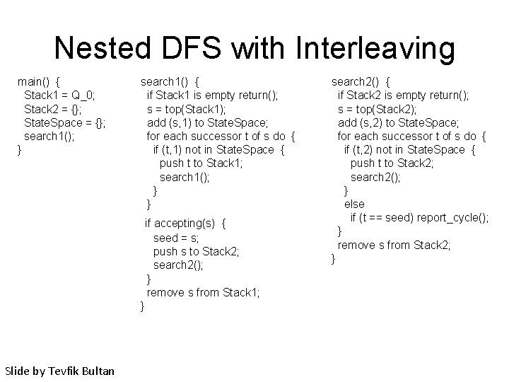
Nested Depth First Search • This algorithm visits each state in the graph once in each depth-first search, and it only needs to mark each visited state – Hence, there is no need to store two integer variables per state, this search can be implemented using one Boolean variable per state. • We can also interleave the first and the second depth-first search. – In the interleaved nested depth first search two Boolean variables per state are used to mark if the stored state is visited during the first search or the second search. Slide by Tevfik Bultan

Nested DFS without Interleaving main() { Stack = Q_0; Queue = {}; State. Space = {}; search 1(); while Queue not empty { s = head(Queue); remove s from Queue; push s to Stack; seed = s; search 2(); } } Slide by Tevfik Bultan search 1() { if Stack is empty return(); s = top(Stack); add (s, 1) to State. Space; for each successor t of s do { if (t, 1) not in State. Space { push t to Stack; search 1(); } } if accepting(s) add s to Queue; remove s from Stack; } search 2() { if Stack is empty return(); s : = top(Stack); add (s, 2) to State. Space; for each successor t of s do if (t, 2) not in State. Space { push t to Stack; search 2(); } else if (t == seed) report_cycle(); remove s from Stack; }

Nested DFS with Interleaving main() { Stack 1 = Q_0; Stack 2 = {}; State. Space = {}; search 1(); } search 1() { if Stack 1 is empty return(); s = top(Stack 1); add (s, 1) to State. Space; for each successor t of s do { if (t, 1) not in State. Space { push t to Stack 1; search 1(); } } if accepting(s) { seed = s; push s to Stack 2; search 2(); } remove s from Stack 1; } Slide by Tevfik Bultan search 2() { if Stack 2 is empty return(); s = top(Stack 2); add (s, 2) to State. Space; for each successor t of s do { if (t, 2) not in State. Space { push t to Stack 2; search 2(); } else if (t == seed) report_cycle(); } remove s from Stack 2; }

The Explicit Stack • Why do we keep an explicit stack during the depth first search (in addition to the control stack that is automatically handled via recursive procedure calls)? • In the report_cycle() procedure we use the contents of Stack 1 and Stack 2 to print the counter-example path – Note that if we print the states in Stack 1 and Stack 2 in the order they are pushed to the stack then we end up printing a counter-example path. Slide by Tevfik Bultan

Bit State Hashing • We are storing visited states in the State. Space – Each state can be inserted to the State. Space twice (once for the first search and once for the second search) • Assume that – we have M bytes of memory – we use K bytes of storage per state – the transition systems has R reachable states • Then the portion of state space we can cover is M / (2 K R) • The idea in bit-state hashing is to improve the coverage of the state space using an hash function – However this may cause us to miss some bugs! Slide by Tevfik Bultan

Bit State Hashing (aka Bloom Filters) • The idea is to use boolean arrays as hash tables and use a hash function to mark these arrays • When we visit a state we will compute the hash value for that state and we will mark the entry that corresponds to the hash value in the hash table as visited • If later on another state is mapped to the same hash value it will not be explored since that entry has been marked as visited • Note that normally we would store the value (i. e. , the state) in the hash table to resolve conflicts. In bit state hashing we are discarding the value to save memory. – When there is a hash collision some states are not explored since the entry corresponding to them are marked as visited earlier by another state. Slide by Tevfik Bultan

Bit State Hashing • Bit state hashing is better than partial depth first search for two reasons: – the states that are ignored during bit state hashing are randomly distributed – we can explore more states using bit state hashing since we are using less memory per state • The portion of state space we can cover using bit state hashing is (M 4) / R – Remember that without bit state hashing the portion of the state space we can cover was M / (2 K R) Slide by Tevfik Bultan

Nested DFS with Interleaving and Bit State Hashing main() { boolean H 1[MAX]; boolean H 2[MAX]; Stack 1 = Q_0; Stack 2 = {}; set H 1 and H 2 to false search 1(); } search 1() { if Stack 1 is empty return(); s = top(Stack 1); H 1[hash(s)] : = true; for each successor t of s do { if H 1[hash(t)] = false { push t to Stack 1; search 1(); } } if accepting(s) { seed = s; push s to Stack 2; search 2(); } remove s from Stack 1; } Slide by Tevfik Bultan search 2() { if Stack 2 is empty return(); s = top(Stack 2); H 2[hash(s)] : = true; for each successor t of s do { if H 2[hash(t)] = false { push t to Stack 2; search 2(); } else if (t == seed) report_cycle(); } remove s from Stack 2; }

Bit State Hashing • Due to bit state hashing we may miss some bugs • However, if we find a bug using bit state hashing, it is a real bug – Bit state hashing will not cause us to report spurious bugs since the states stored in the stacks denote a real execution path Slide by Tevfik Bultan

On-The-Fly Model Checking • In the automata-based model checking: – we are looking for accepting states • that are reachable from an initial state and • that are part of a cycle – in the automaton that corresponds to the product of • the transition system automaton and • the negated property automaton • If we construct the product automaton first and then do the search for accepting cycles, – then we would traverse the whole state space of the transition system while computing the product Slide by Tevfik Bultan

On-The-Fly Model Checking • In on-the-fly model checking we do not construct the product automaton before the search • Instead we construct the product automaton during the nested depth first search • This is what happens: – During the depth first search we execute the transitions of the transition system automaton and the property automaton synchronously to find the successors of a given state – A state is accepting if the property automaton is at an accepting state (all states of the transition system automaton are accepting) Slide by Tevfik Bultan

On-The-Fly Model Checking • This type of on-demand exploration of the state space helps us avoid visiting all the states in case we find an accepting cycle (i. e. , a counter-example behavior) • Note that once we find an accepting cycle we can stop the search and report the counterexample – We do not have to traverse the rest of the state space Slide by Tevfik Bultan

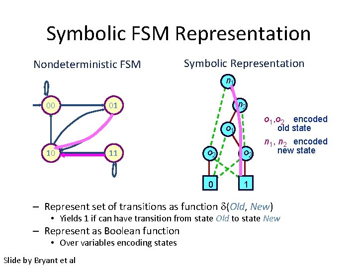
Symbolic Model Checking • Binary Decision Diagrams • Efficient encoding of transition relation and fixpoint computation

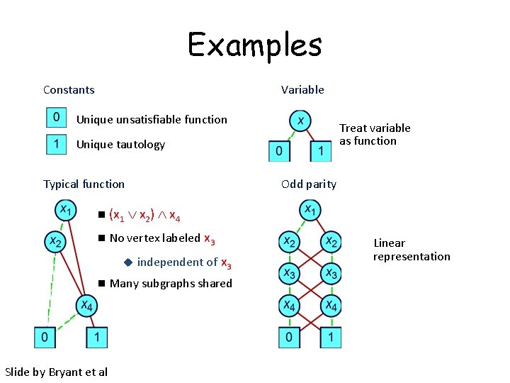
Binary Decision Diagrams -canonical data structure for representing quantifierfree boolean formulas -equivalence checking in constant time -in practice, model checkers spend more than 90% of their time in “pre-image” or “post-image” computation -almost synonymous with “symbolic” model checking -SAT solvers superior in bounded model checking, which requires no termination (i. e. , equivalence) check Slide by Bryant et al

Binary Decision Tree -order k boolean variables x 1, . . . , xk -binary tree of height k+1, each leaf labeled 0 or 1 -leaf of path “left, right, . . . ” gives value of boolean formula if x 1=0, x 2=1, x 3=1, etc. Slide by Bryant et al

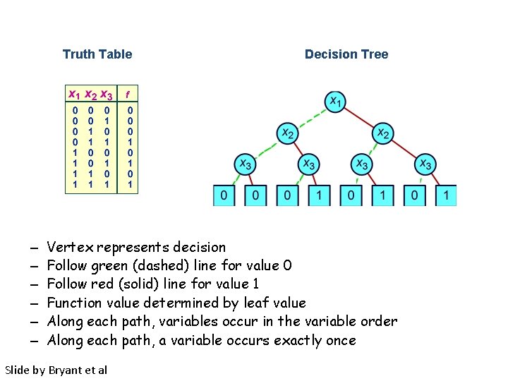
Truth Table – – – Decision Tree Vertex represents decision Follow green (dashed) line for value 0 Follow red (solid) line for value 1 Function value determined by leaf value Along each path, variables occur in the variable order Along each path, a variable occurs exactly once Slide by Bryant et al

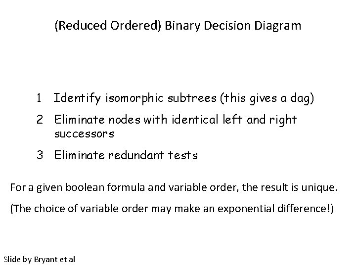
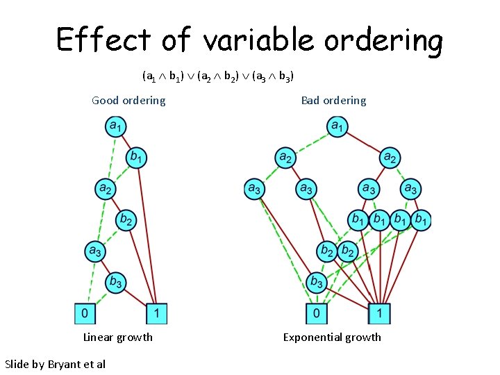
(Reduced Ordered) Binary Decision Diagram 1 Identify isomorphic subtrees (this gives a dag) 2 Eliminate nodes with identical left and right successors 3 Eliminate redundant tests For a given boolean formula and variable order, the result is unique. (The choice of variable order may make an exponential difference!) Slide by Bryant et al

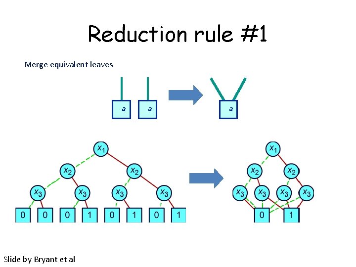
Reduction rule #1 Merge equivalent leaves a Slide by Bryant et al a a

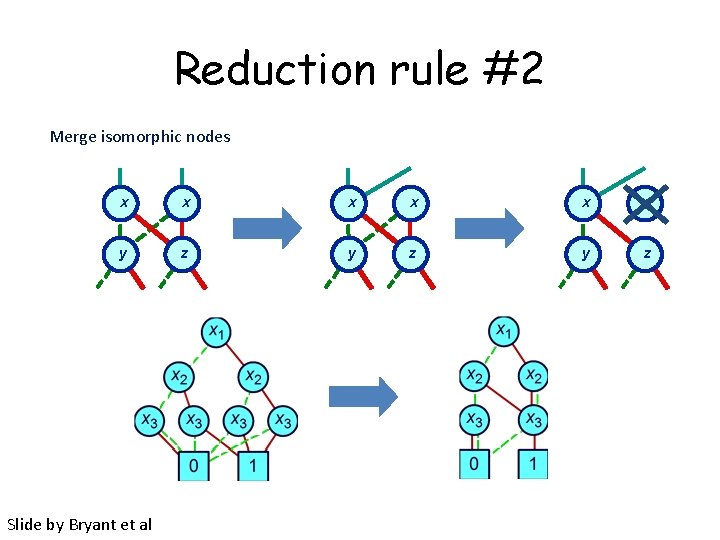
Reduction rule #2 Merge isomorphic nodes x x x y z y z Slide by Bryant et al

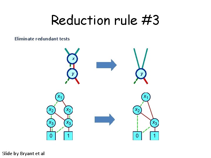
Reduction rule #3 Eliminate redundant tests x y Slide by Bryant et al y

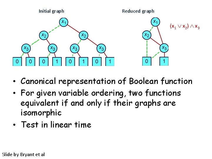
Initial graph Reduced graph (x 1 x 2) x 3 • Canonical representation of Boolean function • For given variable ordering, two functions equivalent if and only if their graphs are isomorphic • Test in linear time Slide by Bryant et al

Examples Constants Variable Unique unsatisfiable function Treat variable as function Unique tautology Odd parity Typical function n (x 1 x 2) x 4 n No vertex labeled x 3 u n Slide by Bryant et al independent of x 3 Many subgraphs shared Linear representation

Effect of variable ordering (a 1 b 1) (a 2 b 2) (a 3 b 3) Good ordering Linear growth Slide by Bryant et al Bad ordering Exponential growth

Dynamic variable reordering • Invented by Richard Rudell, Synopsys • Periodically attempt to improve ordering for all BDDs – Part of garbage collection – Move each variable through ordering to find its best location • Has proved very successful Slide by Bryant et al

Symbolic FSM Representation Nondeterministic FSM Symbolic Representation n 1 00 n 2 01 o 1 10 11 o 2 0 1 o 1, o 2 encoded old state n 1, n 2 encoded new state – Represent set of transitions as function (Old, New) • Yields 1 if can have transition from state Old to state New – Represent as Boolean function • Over variables encoding states Slide by Bryant et al

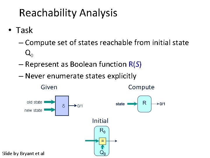
Reachability Analysis • Task – Compute set of states reachable from initial state Q 0 – Represent as Boolean function R(S) – Never enumerate states explicitly Given old state new state Compute 0/1 Initial Slide by Bryant et al

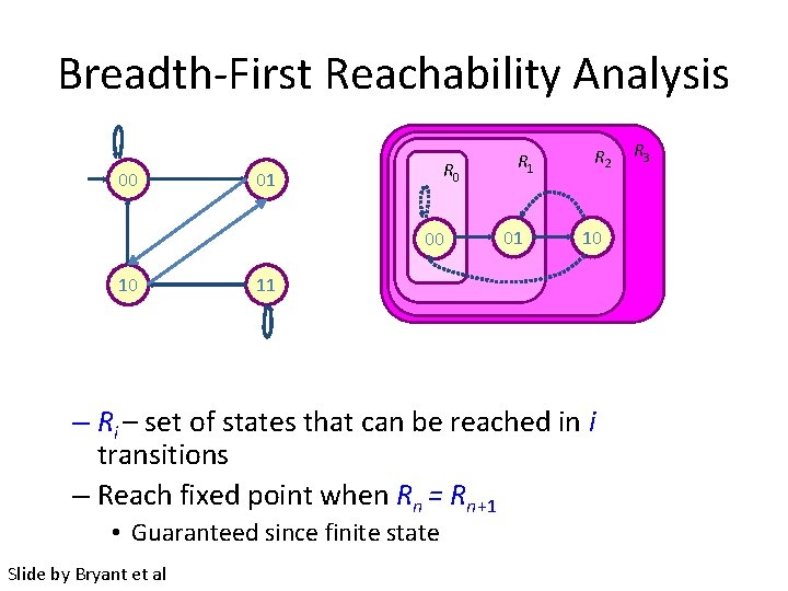
Breadth-First Reachability Analysis 00 R 0 01 00 00 10 R 1 01 R 2 10 11 – Ri – set of states that can be reached in i transitions – Reach fixed point when Rn = Rn+1 • Guaranteed since finite state Slide by Bryant et al R 3

BDD operations , , BDD node n. var = x n. false = a n. true = b n x a b - BDD manager maintains a directed acyclic graph of BDD nodes - ite(x, a, b) returns a node with variable x, left child a, and right child b. Slide by Bryant et al

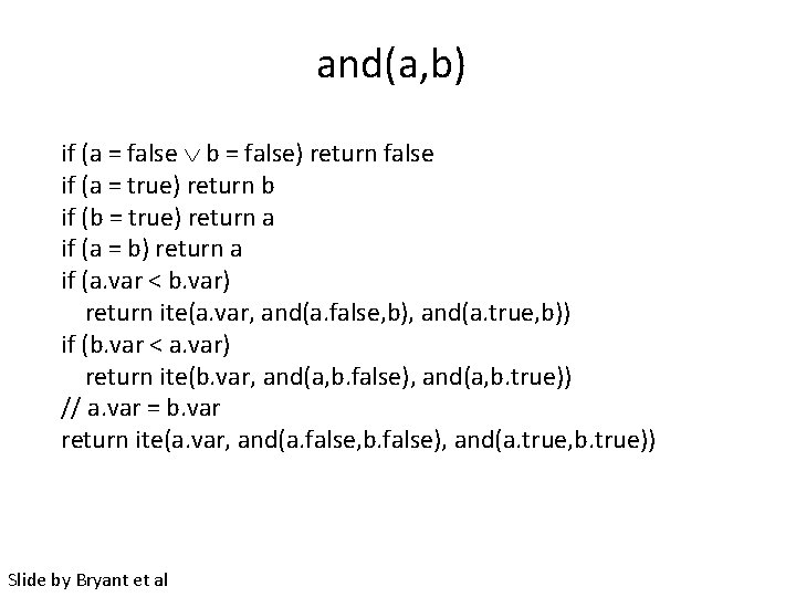
and(a, b) if (a = false b = false) return false if (a = true) return b if (b = true) return a if (a = b) return a if (a. var < b. var) return ite(a. var, and(a. false, b), and(a. true, b)) if (b. var < a. var) return ite(b. var, and(a, b. false), and(a, b. true)) // a. var = b. var return ite(a. var, and(a. false, b. false), and(a. true, b. true)) Slide by Bryant et al

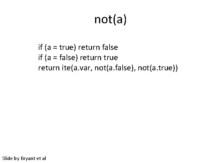
not(a) if (a = true) return false if (a = false) return true return ite(a. var, not(a. false), not(a. true)) Slide by Bryant et al

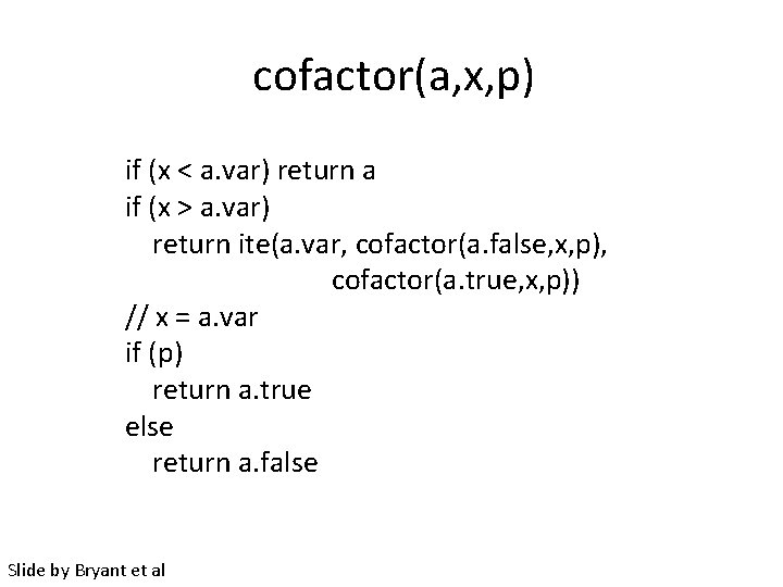
cofactor(a, x, p) if (x < a. var) return a if (x > a. var) return ite(a. var, cofactor(a. false, x, p), cofactor(a. true, x, p)) // x = a. var if (p) return a. true else return a. false Slide by Bryant et al

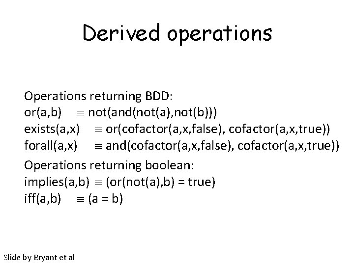
Derived operations Operations returning BDD: or(a, b) not(and(not(a), not(b))) exists(a, x) or(cofactor(a, x, false), cofactor(a, x, true)) forall(a, x) and(cofactor(a, x, false), cofactor(a, x, true)) Operations returning boolean: implies(a, b) (or(not(a), b) = true) iff(a, b) (a = b) Slide by Bryant et al

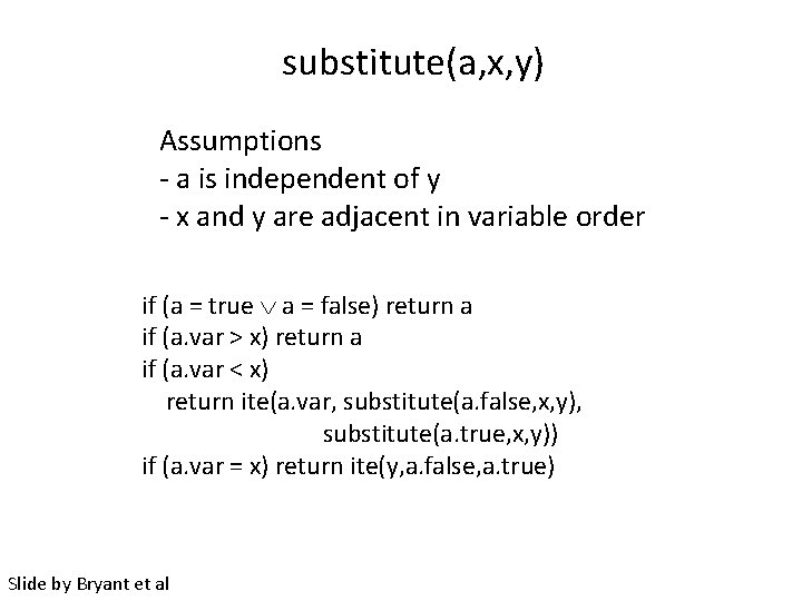
substitute(a, x, y) Assumptions - a is independent of y - x and y are adjacent in variable order if (a = true a = false) return a if (a. var > x) return a if (a. var < x) return ite(a. var, substitute(a. false, x, y), substitute(a. true, x, y)) if (a. var = x) return ite(y, a. false, a. true) Slide by Bryant et al

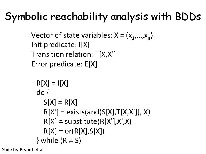
Symbolic reachability analysis with BDDs Vector of state variables: X = (x 1, …, xn) Init predicate: I[X] Transition relation: T[X, X’] Error predicate: E[X] R[X] = I[X] do { S[X] = R[X] R[X’] = exists(and(S[X], T[X, X’]), X) R[X] = substitute(R[X’], X’, X) R[X] = or(R[X], S[X]) } while (R S) Slide by Bryant et al

Bounded Model Checking • BDDs are good for reaching fix points • However if you just unwind transition relation a bounded number of times a SAT check for the property can be more efficient

Remember Symbolic Model Checking • Represent sets of states and the transition relation as Boolean logic formulas • Fixpoint computation becomes formula manipulation – pre-condition (EX) computation: Existential variable elimination – conjunction (intersection), disjunction (union) and negation (set difference), and equivalence check • Use an efficient data structure for boolean logic formulas – Binary Decision Diagrams (BDDs) Slide by Tevfik Bultan

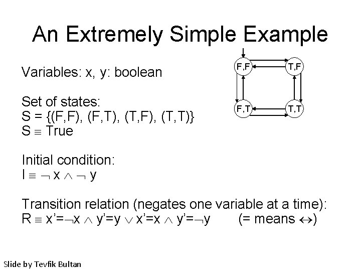
An Extremely Simple Example Variables: x, y: boolean Set of states: S = {(F, F), (F, T), (T, F), (T, T)} S True F, F T, F F, T T, T Initial condition: I x y Transition relation (negates one variable at a time): R x’= x y’=y x’=x y’= y (= means ) Slide by Tevfik Bultan

An Extremely Simple Example • Assume that we want to check if this transition system satisfies the property AG( x y) • Instead of checking AG( x y) we can check EF(x y) – Since AG( x y) EF(x y) I AG( x y) if and only if I EF(x y) = • If we find an initial state which satisfies EF(x y) (i. e. , there exists a path from an initial state where eventually x and y both become true at the same time) – Then we conclude that the property AG( x y) does not hold for this transition system • If there is no such initial state, then property AG( x y) holds for this transition system Slide by Tevfik Bultan

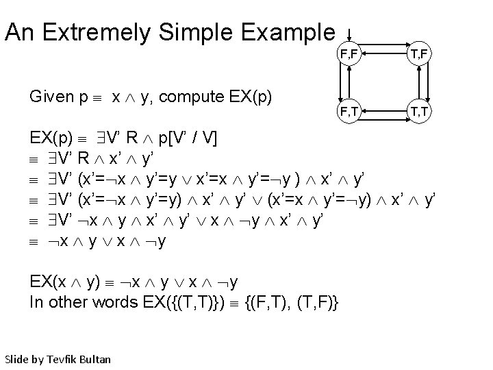
An Extremely Simple Example Given p x y, compute EX(p) F, F T, F F, T T, T EX(p) V’ R p[V’ / V] V’ R x’ y’ V’ (x’= x y’=y x’=x y’= y ) x’ y’ V’ (x’= x y’=y) x’ y’ (x’=x y’= y) x’ y’ V’ x y x’ y’ x y EX(x y) x y In other words EX({(T, T)}) {(F, T), (T, F)} Slide by Tevfik Bultan

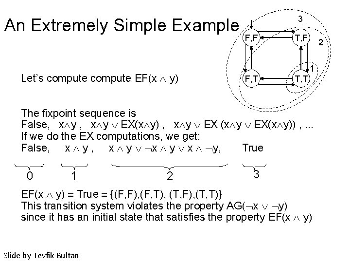
An Extremely Simple Example Let’s compute EF(x y) 3 F, F T, F 2 1 F, T The fixpoint sequence is False, x y EX(x y) , x y EX (x y EX(x y)) , . . . If we do the EX computations, we get: False, x y x y, True 0 1 2 3 EF(x y) True {(F, F), (F, T), (T, F), (T, T)} This transition system violates the property AG( x y) since it has an initial state that satisfies the property EF(x y) Slide by Tevfik Bultan

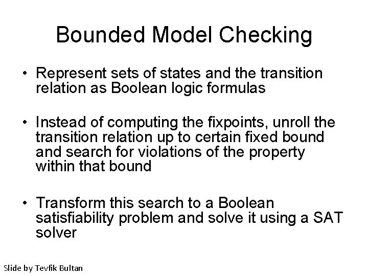
Bounded Model Checking • Represent sets of states and the transition relation as Boolean logic formulas • Instead of computing the fixpoints, unroll the transition relation up to certain fixed bound and search for violations of the property within that bound • Transform this search to a Boolean satisfiability problem and solve it using a SAT solver Slide by Tevfik Bultan

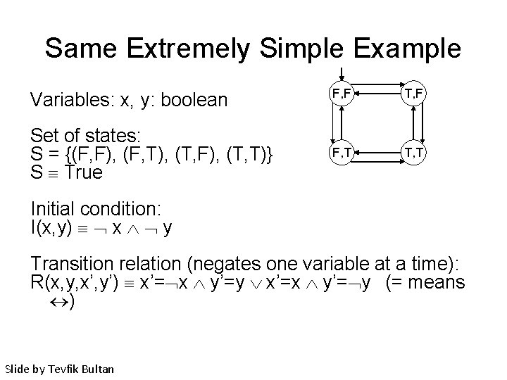
Same Extremely Simple Example Variables: x, y: boolean F, F T, F Set of states: S = {(F, F), (F, T), (T, F), (T, T)} S True F, T T, T Initial condition: I(x, y) x y Transition relation (negates one variable at a time): R(x, y, x’, y’) x’= x y’=y x’=x y’= y (= means ) Slide by Tevfik Bultan

Bounded Model Checking • Assume that we like to check that if the initial states satisfy the formula EF(x y) • Instead of computing a backward fixpoint, we will unroll the transition relation a fixed number of times starting from the initial states • For each unrolling we will create a new set of variables: – The initial states of the system will be characterized with the variables x 0 and y 0 – The states of the system after executing one transition will be characterized with the variables x 1 and y 1 – The states of the system after executing two transitions will be characterized with the variables x 2 and y 2 Slide by Tevfik Bultan

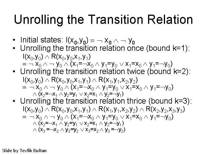
Unrolling the Transition Relation • Initial states: I(x 0, y 0) x 0 y 0 • Unrolling the transition relation once (bound k=1): I(x 0, y 0) R(x 0, y 0, x 1, y 1) x 0 y 0 (x 1= x 0 y 1=y 0 x 1=x 0 y 1= y 0) • Unrolling the transition relation twice (bound k=2): I(x 0, y 0) R(x 0, y 0, x 1, y 1) R(x 1, y 1, x 2, y 2) x 0 y 0 (x 1= x 0 y 1=y 0 x 1=x 0 y 1= y 0) (x 2= x 1 y 2=y 1 x 2=x 1 y 2= y 1) • Unrolling the transition relation thrice (bound k=3): I(x 0, y 0) R(x 0, y 0, x 1, y 1) R(x 1, y 1, x 2, y 2) R(x 2, y 2, x 3, y 3) x 0 y 0 (x 1= x 0 y 1=y 0 x 1=x 0 y 1= y 0) (x 2= x 1 y 2=y 1 x 2=x 1 y 2= y 1) (x 3 = x 2 y 3=y 2 x 3=x 2 y 3 = y 2) Slide by Tevfik Bultan

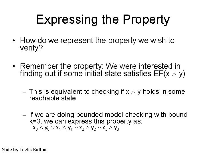
Expressing the Property • How do we represent the property we wish to verify? • Remember the property: We were interested in finding out if some initial state satisfies EF(x y) – This is equivalent to checking if x y holds in some reachable state – If we are doing bounded model checking with bound k=3, we can express this property as: x 0 y 0 x 1 y 1 x 2 y 2 x 3 y 3 Slide by Tevfik Bultan

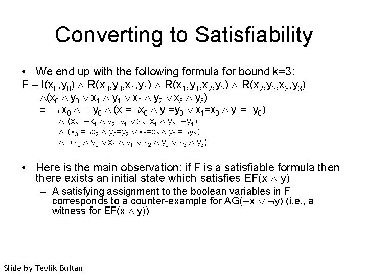
Converting to Satisfiability • We end up with the following formula for bound k=3: F I(x 0, y 0) R(x 0, y 0, x 1, y 1) R(x 1, y 1, x 2, y 2) R(x 2, y 2, x 3, y 3) (x 0 y 0 x 1 y 1 x 2 y 2 x 3 y 3) x 0 y 0 (x 1= x 0 y 1=y 0 x 1=x 0 y 1= y 0) (x 2= x 1 y 2=y 1 x 2=x 1 y 2= y 1) (x 3 = x 2 y 3=y 2 x 3=x 2 y 3 = y 2) (x 0 y 0 x 1 y 1 x 2 y 2 x 3 y 3) • Here is the main observation: if F is a satisfiable formula then there exists an initial state which satisfies EF(x y) – A satisfying assignment to the boolean variables in F corresponds to a counter-example for AG( x y) (i. e. , a witness for EF(x y)) Slide by Tevfik Bultan

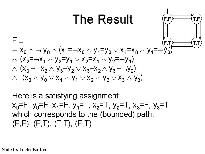
The Result F, F F F, T x 0 y 0 (x 1= x 0 y 1=y 0 x 1=x 0 y 1= y 0) (x 2= x 1 y 2=y 1 x 2=x 1 y 2= y 1) (x 3 = x 2 y 3=y 2 x 3=x 2 y 3 = y 2) (x 0 y 0 x 1 y 1 x 2 y 2 x 3 y 3) Here is a satisfying assignment: x 0=F, y 0=F, x 1=F, y 1=T, x 2=T, y 2=T, x 3=F, y 3=T which corresponds to the (bounded) path: (F, F), (F, T), (T, T), (F, T) Slide by Tevfik Bultan T, F T, T

What Can We Guarantee? • We converted checking property AG(p) to Boolean SAT solving by looking for bounded paths that satisfy EF( p) • Note that we are checking only for bounded paths (paths which have at most k+1 distinct states) – So if the property is violated by only paths with more than k+1 distinct states, we would not find a counter-example using bounded model checking – Hence if we do not find a counter-example using bounded model checking we are not sure that the property holds • However, if we find a counter-example, then we are sure that the property is violated since the generated counter-example is never spurious (i. e. , it is always a concrete counter-example) Slide by Tevfik Bultan

Bounded Model Checking for LTL • It is possible to extend the basic ideas we discussed for verifying properties of the form AG(p) to all LTL properties. • The basic observation is that we can define a bounded semantics for LTL properties so that if a path satisfies an LTL property based on the bounded semantics, then it satisfies the property based on the unbounded semantics – This is why a counter-example found on a bounded path is guaranteed to be a real counter-example – However, this does not guarantee correctness Slide by Tevfik Bultan

Bounded Model Checking: Proving Correctness • One can also show that given an LTL property f, if E f holds for a finite state transition system, then E f also holds for that transition system using bounded semantics for some bound k • So if we keep increasing the bound, then we are guaranteed to find a path that satisfies the formula – And, if we do not find a path that satisfies the formula, then we decide that the formula is not satisfied by the transition system – Is there a problem here? Slide by Tevfik Bultan

Proving Correctness • We can modify the bounded model checking algorithm as follows: – Start from an initial bound. – If no counter-examples are found using the current bound, increment the bound and try again. • The problem is: – We do not know when to stop Slide by Tevfik Bultan

Proving Correctness • If we can find a way to figure out when we should stop then we would be able to provide guarantee of correctness. • There is a way to define a diameter of a transition system so that a property holds for the transition system if and only if it is not violated on a path bounded by the diameter. • So if we do bounded model checking using the diameter of the system as our bound, then we can guarantee correctness if no counter-example is found. Slide by Tevfik Bultan

Bounded Model Checking • What are the differences between bounded model checking and BDD-based symbolic model checking? – In bounded model checking we are using a SAT solver instead of a BDD library – In symbolic model checking we do not unroll the transition relation as in bounded model checking – In bounded model checking we do not compute the fixpoint as in symbolic model checking – In symbolic model checking for finite state systems both verification and falsification results are guaranteed • In bounded model checking we can only guarantee the falsification results, in order to guarantee the verification results we need to know the diameter of the system Slide by Tevfik Bultan

Bounded Model Checking • Boolean satisfiability problem (SAT) is an NP-complete problem • A bounded model checker needs an efficient SAT solver – z. Chaff SAT solver is one of the most commonly used ones – However, in the worst case any SAT solver we know will take exponential time • Most SAT solvers require their input to be in Conjunctive Normal Form (CNF) – So the final formula has to be converted to CNF Slide by Tevfik Bultan

Bounded Model Checking • Similar to BDD-based symbolic model checking, bounded model checking was also first used for hardware verification • Later on, it was applied to software verification Slide by Tevfik Bultan

Overview • • • A Brief History of Model Checking My History of Model Checking The Models of Model Checking Temporal Logic Algorithms for Model Checking Retrospective

LTL versus CTL • Another approach to classify model checking algorithms is to look at the type of properties that can be checked

LTL Model Checking • Given a transition system T and an LTL property p T |= p iff for all execution paths x in T, x |= p For example: T |=? G ( (pc 1=c pc 2=c)) T |=? G(pc 1=w F(pc 1=c)) G(pc 2=w F(pc 2=c)) Model checking problem: Given a transition system T and an LTL property p, determine if T is a model for p (i. e. , if T |=p) Slide by Tevfik Bultan

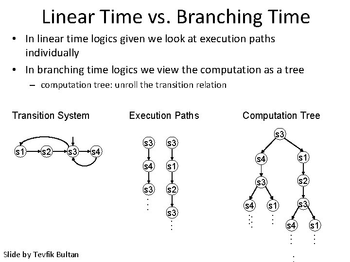
Linear Time vs. Branching Time • In linear time logics given we look at execution paths individually • In branching time logics we view the computation as a tree – computation tree: unroll the transition relation Transition System s 1 s 2 s 3 Execution Paths s 4 s 3. . . s 3 s 1 s 2 s 3. . . Slide by Tevfik Bultan Computation Tree s 4. . . s 4 s 1 s 3 s 2 s 3 s 1. . . s 4. . s 1. . .

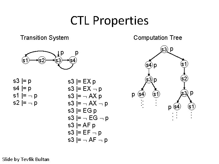
CTL Properties Transition System p s 1 s 2 s 3 |= p s 4 |= p s 1 |= p s 2 |= p Slide by Tevfik Bultan s 3 Computation Tree s 3 p p s 4 s 3 |= EX p s 3 |= EX p s 3 |= AX p s 3 |= EG p s 3 |= EG p s 3 |= AF p s 3 |= EF p s 3 |= AF p p s 4. . . s 4 p s 1 s 3 p s 2 s 3 p s 1. . . p s 4. . . s 1. . .

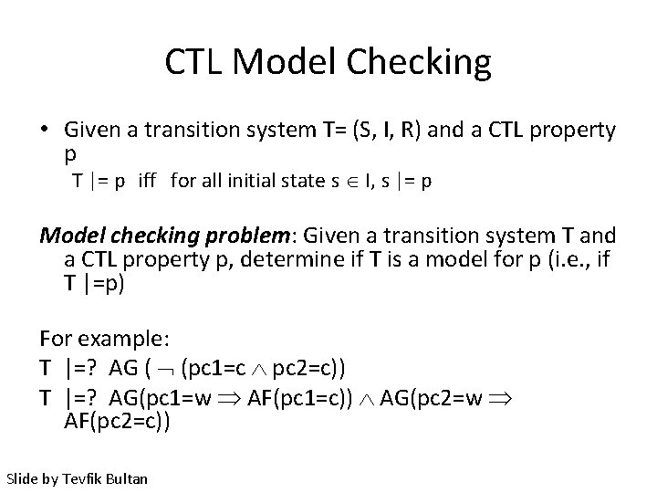
CTL Model Checking • Given a transition system T= (S, I, R) and a CTL property p T |= p iff for all initial state s I, s |= p Model checking problem: Given a transition system T and a CTL property p, determine if T is a model for p (i. e. , if T |=p) For example: T |=? AG ( (pc 1=c pc 2=c)) T |=? AG(pc 1=w AF(pc 1=c)) AG(pc 2=w AF(pc 2=c)) Slide by Tevfik Bultan

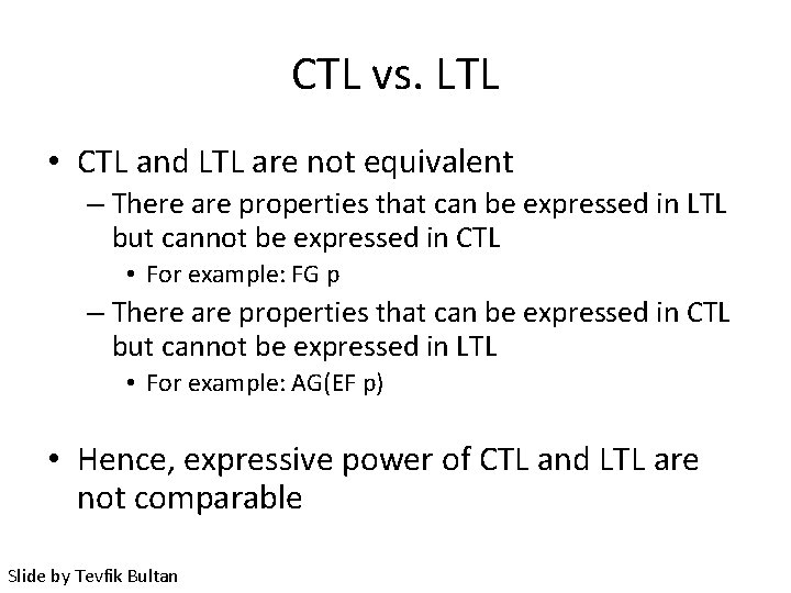
CTL vs. LTL • CTL and LTL are not equivalent – There are properties that can be expressed in LTL but cannot be expressed in CTL • For example: FG p – There are properties that can be expressed in CTL but cannot be expressed in LTL • For example: AG(EF p) • Hence, expressive power of CTL and LTL are not comparable Slide by Tevfik Bultan

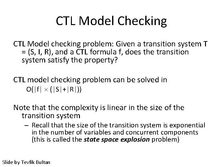
CTL Model Checking CTL Model checking problem: Given a transition system T = (S, I, R), and a CTL formula f, does the transition system satisfy the property? CTL model checking problem can be solved in O(|f| (|S|+|R|)) Note that the complexity is linear in the size of the transition system – Recall that the size of the transition system is exponential in the number of variables and concurrent components (this is called the state space explosion problem) Slide by Tevfik Bultan

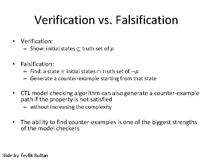
Verification vs. Falsification • Verification: – Show: initial states truth set of p • Falsification: – Find: a state initial states truth set of p – Generate a counter-example starting from that state • CTL model checking algorithm can also generate a counter-example path if the property is not satisfied – without increasing the complexity • The ability to find counter-examples is one of the biggest strengths of the model checkers Slide by Tevfik Bultan

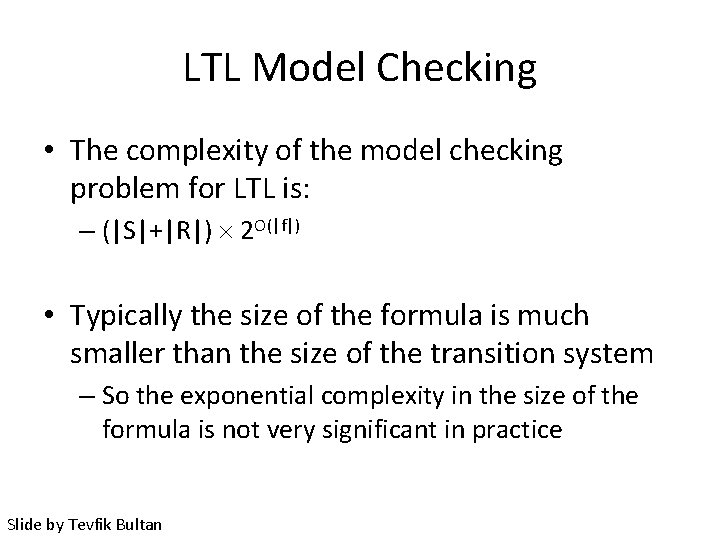
LTL Model Checking • The complexity of the model checking problem for LTL is: – (|S|+|R|) 2 O(|f|) • Typically the size of the formula is much smaller than the size of the transition system – So the exponential complexity in the size of the formula is not very significant in practice Slide by Tevfik Bultan

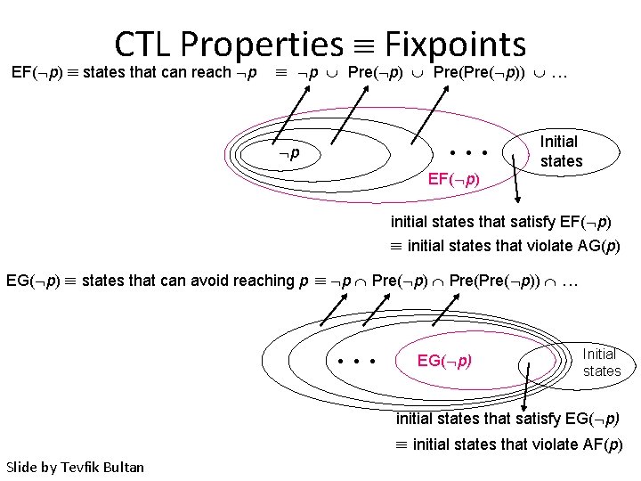
CTL Properties Fixpoints EF( p) states that can reach p p Pre( p)) . . . p • • • EF( p) Initial states initial states that satisfy EF( p) initial states that violate AG(p) EG( p) states that can avoid reaching p p Pre( p)) . . . • • • EG( p) Initial states initial states that satisfy EG( p) initial states that violate AF(p) Slide by Tevfik Bultan

Symbolic Model Checking • Represent sets of states and the transition relation as Boolean logic formulas • Fixpoint computation becomes formula manipulation – pre and post-condition computations: Existential variable elimination – conjunction (intersection), disjunction (union) and negation (set difference), and equivalence check • Use an efficient data structure – Binary Decision Diagrams (BDDs) Slide by Tevfik Bultan

SMV • • A BDD-based symbolic model checker Finite state Temporal logic: CTL Focus: hardware verification – Later applied to software specifications, protocols, etc. • SMV has its own input specification language – – concurrency: synchronous, asynchronous shared variables boolean and enumerated variables bounded integer variables (binary encoding) • SMV is not efficient for integers, but it can be fixed – fixed size arrays Slide by Tevfik Bultan

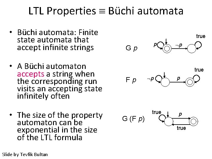
LTL Properties Büchi automata • Büchi automata: Finite state automata that accept infinite strings • A Büchi automaton accepts a string when the corresponding run visits an accepting state infinitely often • The size of the property automaton can be exponential in the size of the LTL formula Slide by Tevfik Bultan true Gp p p true Fp G (F p) p true p p true

Automata Based Model Checking • Generate a property automaton from the negated LTL property • Take the product of the property automaton and the transition system • Look for an accepting cycle in the product automaton • Use a nested depth first search to look for accepting cycles • If there is a cycle, it corresponds to a counterexample behavior that demonstrates a bug Slide by Tevfik Bultan

SPIN • • An explicit state model checker Finite state Temporal logic: LTL Input language: PROMELA – Asynchronous processes – Shared variables – Message passing through (bounded) communication channels – Variables: boolean, char, integer (bounded), arrays (fixed size) – Structured data types Slide by Tevfik Bultan

SPIN Verification in SPIN • An automata based LTL model checker • Constructs the product automaton on-the-fly – It is possible to find a counter-example without constructing the whole state space • Uses various heuristics to improve the efficiency of the search: – partial order reduction – state compression Slide by Tevfik Bultan