Model Atmosphere Codes ATLAS 9 and ATLAS 12

Model Atmosphere Codes: ATLAS 9 and ATLAS 12 Robert L. Kurucz Harvard-Smithsonian Center for Astrophysics 60 Garden Street, Cambridge, MA, USA I present three different treatments of the opacity and the corresponding programs: Resolved spectra and SYNTHE, Sampled spectra and ATLAS 12, and Low resolution distribution functions and DFSYNTHE and ATLAS 9. 1

SYNTHE works in Doppler space so the computed points are uniformly spaced in velocity. For a given species there are the same number of points per Doppler width no matter what the wavelength. A Doppler shift anywhere in the spectrum is a shift by the same number of points so radial velocities are just point number shifts. SYNTHE works only in high resolution because of various approximations that greatly reduce the computation time. By default line centers are moved to the nearest computation point and lines have symmetric Voigt profiles. Other profiles can be used that are not shifted. 2

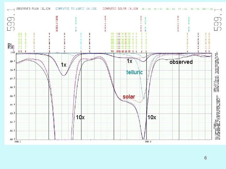
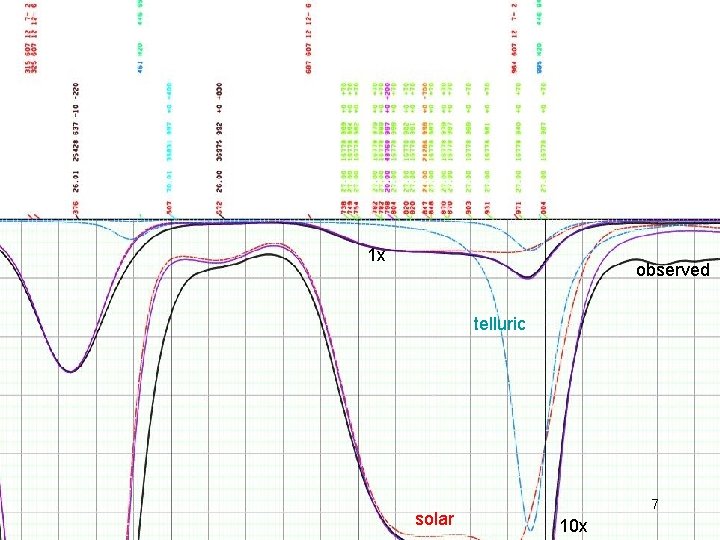
I normally use a resolving power of 500000 for stars and 2000000 for the sun. For really critical work, such as blending solar and telluric lines, I have used resolving powers as high as 10 million since the telluric lines are only 300 K wide. Once I obtain a high resolution spectrum it is easy to broaden it with a Gaussian or other profile (using BROADEN) to any lower resolution, or to many lower resolutions, at low computational cost. 3

SYNTHE was written to work at high resolution with the wavelengths and ionization edges put in as accurately as they have been measured, including the multiplet structure of the edges. It can treat series of lines merging into continua. H, He, C, Mg, Al, Si go to at least n = 80. (ATLAS 12 is the same but ATLAS 9 is inherently low resolution with approximate edges. ) SYNTHE can treat any number of lines. SYNTHE writes out the data for all lines that it uses that are significant, that have a depth greater than 0. 001 (or 0. 0001) of the continuum at any level in the atmosphere. The gf values, damping constants, and wavelengths of these lines can be hand-edited and fed back into the program to iterate on the computed spectrum. This is the mechanism for hand fitting a spectrum. 4

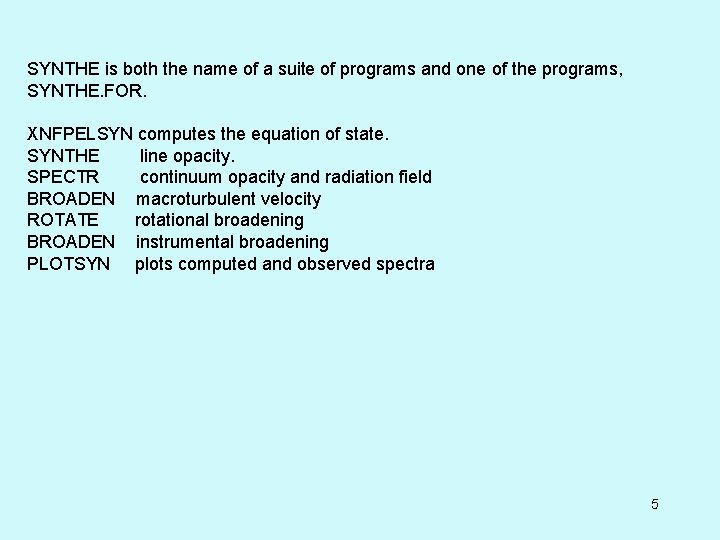
SYNTHE is both the name of a suite of programs and one of the programs, SYNTHE. FOR. XNFPELSYN computes the equation of state. SYNTHE line opacity. SPECTR continuum opacity and radiation field BROADEN macroturbulent velocity ROTATE rotational broadening BROADEN instrumental broadening PLOTSYN plots computed and observed spectra 5

1 x 1 x observed telluric solar 10 x 6

1 x observed telluric solar 7 10 x

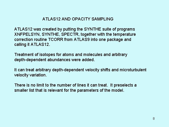
ATLAS 12 AND OPACITY SAMPLING ATLAS 12 was created by putting the SYNTHE suite of programs XNFPELSYN, SYNTHE, SPECTR, together with the temperature correction routine TCORR from ATLAS 9 into one package and calling it ATLAS 12. Treatment of isotopes for atoms and molecules and arbitrary depth-dependent abundances were added. It can treat arbitrary depth-dependent velocity shifts and microturbulent velocity variation. There is no limit to the number of lines it can treat. It preselects a smaller list that is relevant for the parameters of the model. 8

It saves a list of all the lines it actually uses in the calculation in packed form. That list can be used as the input for other similar models or for models with lower abundances. It can also be used to compute spectra. For example, there is a packed line list for models like the sun. That packed line list can be read into SYNTHE using program RPACKEDLINE to generate a high resolution spectrum. 9

There are two types of line data input into ATLAS 12. There are good lines between laboratory energy levels that have reliable wavelengths with relatively small errors. They can be compared to observed spectra and should give good positions and radial velocities. However, the vast majority of lines are between predicted levels and their wavelengths are wrong. But, they increase the opacity. Integrated, the errors in their equivalent widths may average out. Spectra computed with only good lines should be better looking and better cross-correlating but they should produce worse spectrophotometry than spectra computed with both good and predicted lines. I recommend computing the spectra both ways and comparing the two to estimate how much work still needs to be done on the line data. 10

ATLAS 12 can deal with more than 1 billion lines by sampling. It defaults to 30000 sampling points but it could sample more than 1 million. Sampling ranges shift redward as Teff decreases nulo = 1= 10 nm - 10 microns Teff < 30000 nulo = nu. He. II = 3577 = 22. 8 Teff < 13000 nulo = nu. He. I = 7027 = 50. 4 Teff < 7250 nulo = nu. Lyman = 9599 = 91. 1 Teff < 4500 nulo = nu. CI = 11601 = 124. 0 nuhi = nulo+29999 Do nu=1, 30000 wavelength = 10. d 0**(1. do+0. 0001 d 0*(nu+nulo -1)) 11

30000 point sampling is adequate for computing the total flux and a flux constant model but it is not good enough for computing detailed fluxes for comparison with observation. Either the sample has to be larger to reduce the statistical uncertainty or SYNTHE has to be used with the model to compute the spectrum monochromatically. 12

Schematic distribution functions

14

16

17

DFSYNTHE AND ATLAS 9 ODF tables can be found on the web for various abundances and can be interpolated to others. It is not necessary to run DFSYNTHE to compute ATLAS 9 models. ATLAS 9 is suitable for computing grids of models with fixed abundances. Once the ODFs have been computed the cost of computing individual models is low. One can compute grids with hundreds or thousands of models. 18

DFSYNTHE DETAILS DFSYNTHE is a version of SYNTHE that is set up to use a T-P, or T-Ne, or T-density table instead of a model. There might be, say, 50 Ts and 30 Ps. It does one temperature at a time and runs through all the pressures. All the variables that depend only on T such as Boltzman factors are evaluated only once. 19

It has various tricks to reduce the amount of computation. For each T, for each species, it determines the maximum population among the whole range of pressures. Then it reads the whole line list and checks each line to see if Nmax*gf*Boltzman > cutoff. If it is the line is written to a new, smaller linelist that is used as input for each P. At high T molecules are automatically eliminated. At low T high ions are eliminated and high energy levels. 20

Then using the small linelist DFSYNTHE cycles through the pressures and generates a spectrum at up to 4 million points by adding the profile of each line to a buffer. For each line it starts at line center, computes the line center opacity, and adds it to the buffer. It checks whether the line is less than 0. 001 of the continuum opacity. If it is, it goes to the next line. If not, it proceeds outward through the red and blue wings of the Voigt profile until the wing becomes weak, less than 0. 001 of the continuum level. Other types of profiles can be treated explicitly. 21

After reading through the line list DFSYNTHE can write out the opacity spectrum, say 4 million points. This spectrum has no microturbulent broadening, Vturb = 0. By Fourier transforming the spectrum, broadening it, and transforming back, one can generate a series of spectra for various Vturb. By adding the extra variable, one allows interpolating as a function of Vturb. The spectra are divided into wavelength intervals and a distribution function is computed for each Interval. A 4 million point spectrum can be reduced to 12 numbers per interval, or a few thousand numbers for the whole spectrum. 22

After cycling through all the pressures and temperatures and sorting the output file, the result is distribution function tables as a function of T and P and Vturb over the whole spectrum. Alternatively, one can save the spectra and have (say 4 million) monochromatic opacity tables. Or they can be processed in other ways, such as averaging (in the log) in blocks of 100, to produce a lower resolution opacity table with, say, 40000 frequencies. 23

24