MixedSignal Operations TsungChu Huang NCUE Taiwan Outline Operational

Mixed-Signal Operations Tsung-Chu Huang NCUE, Taiwan

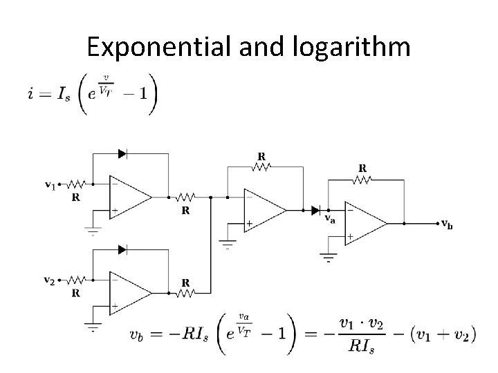
Outline • • • Operational Amplifier Sense Amplifier ADC/DAC Analog Sum/Subtract Analog Exponential/Logarithm Analog Multiplier/Divider Integrator/Differential Delayline Digitalization

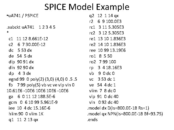
SPICE Model Example • u. A 741 / PSPICE. subckt u. A 741 1 2 3 4 5 * c 1 11 12 8. 661 E-12 c 2 6 7 30. 00 E-12 dc 5 53 dx de 54 5 dx dlp 90 91 dx dln 92 90 dx dp 4 3 dx egnd 99 0 poly(2) (3, 0) (4, 0) 0. 5. 5 fb 7 99 poly(5) vb vc ve vlp vln 0 10. 61 E 6 -10 E 6 -10 E 6 ga 6 0 11 12 188. 5 E-6 gcm 0 6 10 99 5. 961 E-9 iee 10 4 dc 15. 16 E-6 hlim 90 0 vlim 1 K q 1 11 2 13 qx q 2 12 1 14 qx r 2 6 9 100. 0 E 3 rc 1 3 11 5. 305 E 3 rc 2 3 12 5. 305 E 3 re 1 13 10 1. 836 E 3 re 2 14 10 1. 836 E 3 ree 10 99 13. 19 E 6 ro 1 8 5 50 ro 2 7 99 100 rp 3 4 18. 16 E 3 vb 9 0 dc 0 vc 3 53 dc 1 ve 54 4 dc 1 vlim 7 8 dc 0 vlp 91 0 dc 40 vln 0 92 dc 40. model dx D(Is=800. 0 E-18 Rs=1). model qx NPN(Is=800. 0 E-18 Bf=93. 75). ends

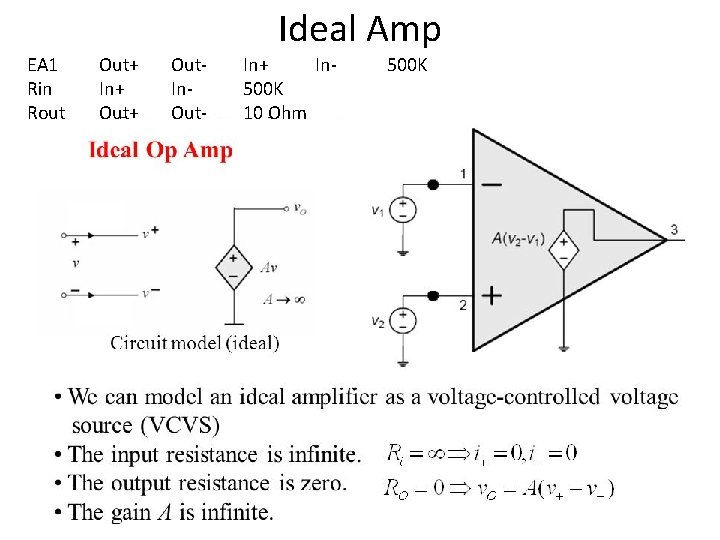
Ideal Amp EA 1 Rin Rout Out+ In+ Out. In. Out- In+ In 500 K 10 Ohm 500 K

A/D Converter (ADC) Introduction • A/D Fundamentals – Sampling – Quantization • Factors Affecting A/D Converter Performance – Static Performance – Dynamic Performance • ADC Architectures – – SAR ADCs Pipelined ADCs Flash Type ADC Sigma-Delta ADCs • High Speed ADC Application Considerations

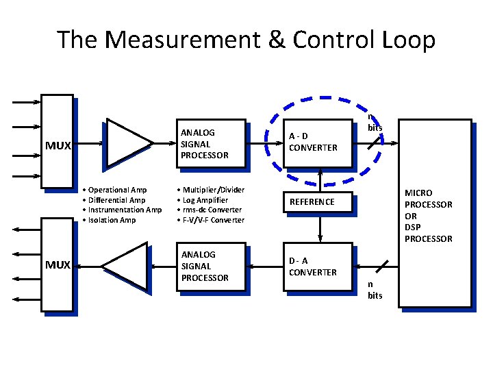
The Measurement & Control Loop ANALOG SIGNAL PROCESSOR MUX • Operational Amp • Differential Amp • Instrumentation Amp • Isolation Amp MUX • Multiplier/Divider • Log Amplifier • rms-dc Converter • F-V/V-F Converter ANALOG SIGNAL PROCESSOR A-D CONVERTER n bits MICRO PROCESSOR OR DSP PROCESSOR REFERENCE D-A CONVERTER n bits

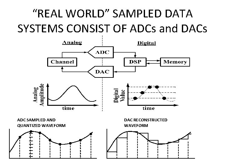
“REAL WORLD” SAMPLED DATA SYSTEMS CONSIST OF ADCs and DACs ADC SAMPLED AND QUANTIZED WAVEFORM DAC RECONSTRUCTED WAVEFORM

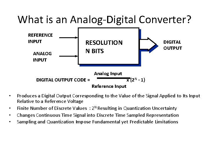
What is an Analog-Digital Converter? REFERENCE INPUT ANALOG INPUT RESOLUTION N BITS DIGITAL OUTPUT CODE = • • Analog Input Reference Input DIGITAL OUTPUT x (2 N - 1) Produces a Digital Output Corresponding to the Value of the Signal Applied to Its Input Relative to a Reference Voltage Finite Number of Discrete Values : 2 N Resulting in Quantization Uncertainty Changes Continuous Time Signal into Discrete Time Sampled Representation Sampling and Quantization Impose Fundamental yet Predictable Limitations

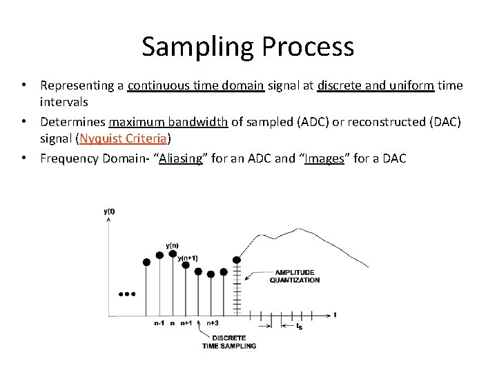
Sampling Process • Representing a continuous time domain signal at discrete and uniform time intervals • Determines maximum bandwidth of sampled (ADC) or reconstructed (DAC) signal (Nyquist Criteria) • Frequency Domain- “Aliasing” for an ADC and “Images” for a DAC

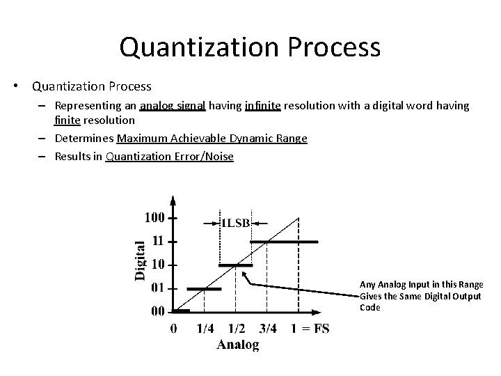
Quantization Process • Quantization Process – Representing an analog signal having infinite resolution with a digital word having finite resolution – Determines Maximum Achievable Dynamic Range – Results in Quantization Error/Noise Any Analog Input in this Range Gives the Same Digital Output Code

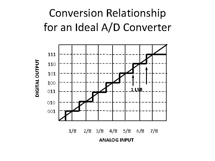
Conversion Relationship for an Ideal A/D Converter DIGITAL OUTPUT 111 110 101 100 1 LSB 011 010 001 1/8 2/8 3/8 4/8 5/8 ANALOG INPUT 6/8 7/8

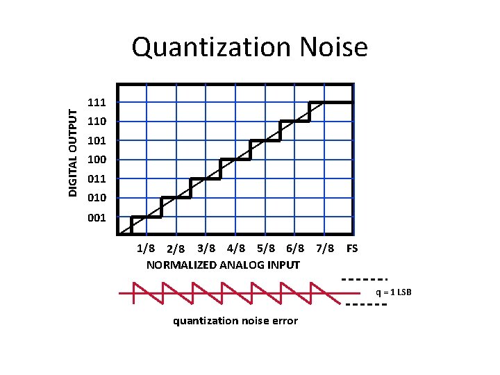
DIGITAL OUTPUT Quantization Noise 111 110 101 100 011 010 001 1/8 2/8 3/8 4/8 5/8 6/8 7/8 NORMALIZED ANALOG INPUT FS q = 1 LSB quantization noise error

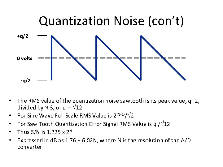
Quantization Noise (con’t) +q/2 0 volts -q/2 • The RMS value of the quantization noise sawtooth is its peak value, q¸ 2, divided by Ö 3, or q ¸ Ö 12 • For Sine Wave Full Scale RMS Value is 2(N-1)/Ö 2 • For Saw Tooth Quantization Error Signal RMS Value is q /Ö 12 • Thus S/N is 1. 225 x 2 N • Expressed in d. B as 1. 76 + 6. 02 N, where N is the resolution of the A/D converter

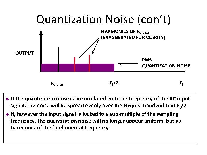
Quantization Noise (con’t) HARMONICS OF FSIGNAL (EXAGGERATED FOR CLARITY) OUTPUT RMS QUANTIZATION NOISE FSIGNAL u If FS/2 FS the quantization noise is uncorrelated with the frequency of the AC input signal, the noise will be spread evenly over the Nyquist bandwidth of F s/2. u If, however the input signal is locked to a sub-multiple of the sampling frequency, the quantization noise will no longer appear uniform, but as harmonics of the fundamental frequency

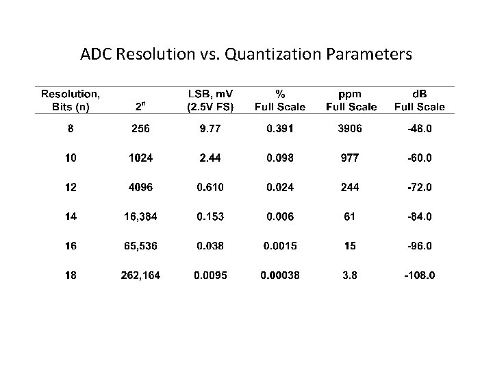
ADC Resolution vs. Quantization Parameters

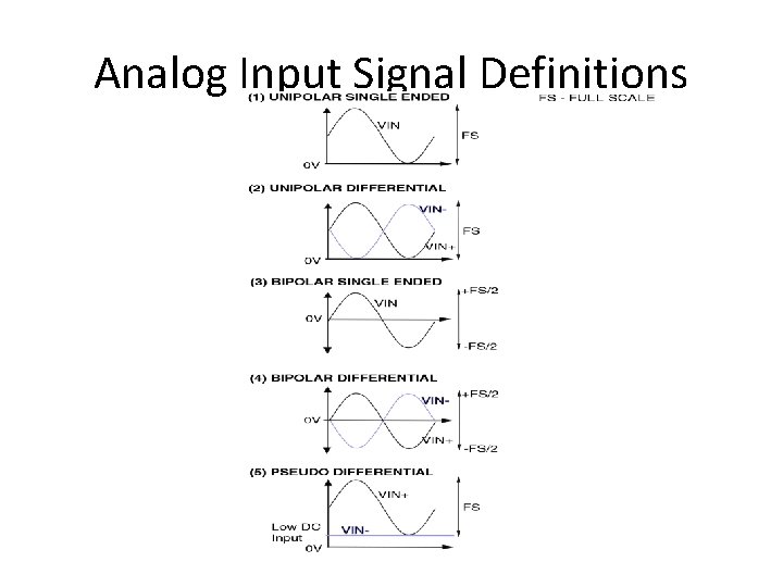
Analog Input Signal Definitions

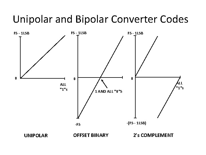
Unipolar and Bipolar Converter Codes FS - 1 LSB 0 0 ALL "1"s 1 AND ALL "0"S -FS UNIPOLAR ALL "1"s OFFSET BINARY -(FS - 1 LSB) 2’s COMPLEMENT

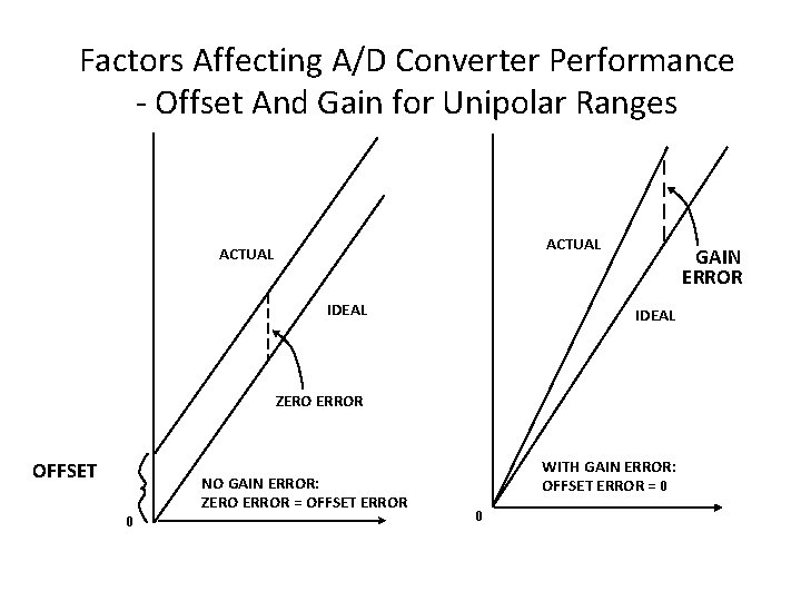
Factors Affecting A/D Converter Performance - Offset And Gain for Unipolar Ranges ACTUAL IDEAL GAIN ERROR IDEAL ZERO ERROR OFFSET 0 NO GAIN ERROR: ZERO ERROR = OFFSET ERROR WITH GAIN ERROR: OFFSET ERROR = 0 0

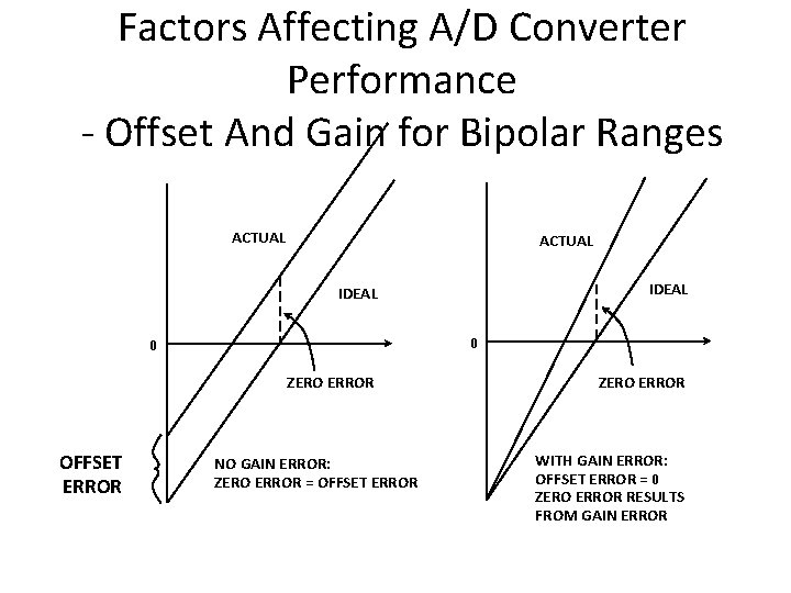
Factors Affecting A/D Converter Performance - Offset And Gain for Bipolar Ranges ACTUAL IDEAL 0 0 ZERO ERROR OFFSET ERROR NO GAIN ERROR: ZERO ERROR = OFFSET ERROR ZERO ERROR WITH GAIN ERROR: OFFSET ERROR = 0 ZERO ERROR RESULTS FROM GAIN ERROR

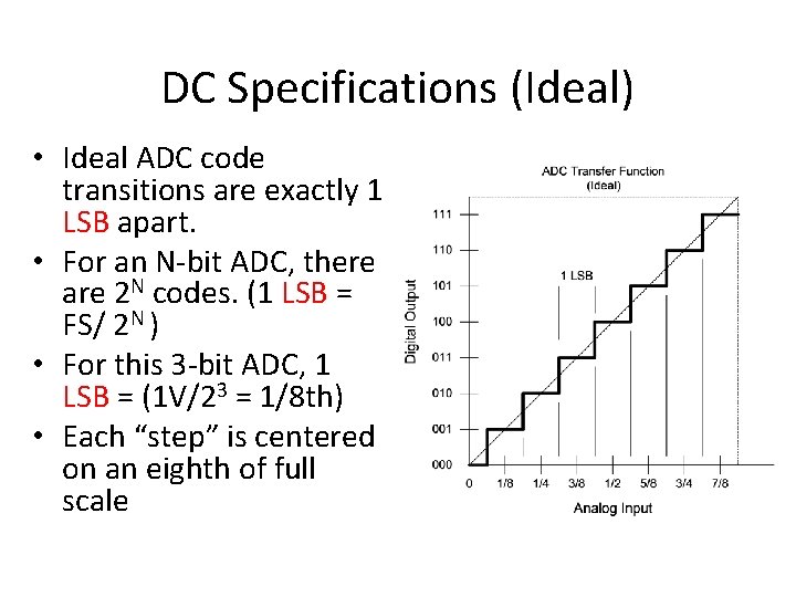
DC Specifications (Ideal) • Ideal ADC code transitions are exactly 1 LSB apart. • For an N-bit ADC, there are 2 N codes. (1 LSB = FS/ 2 N ) • For this 3 -bit ADC, 1 LSB = (1 V/23 = 1/8 th) • Each “step” is centered on an eighth of full scale

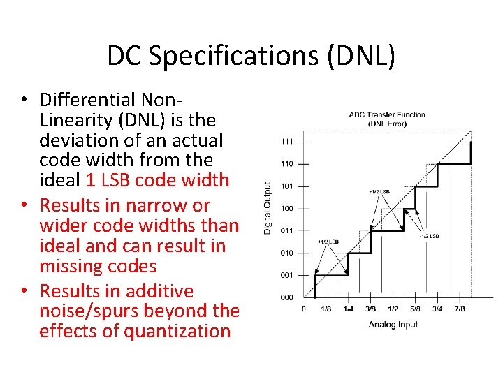
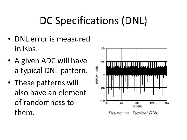
DC Specifications (DNL) • Differential Non. Linearity (DNL) is the deviation of an actual code width from the ideal 1 LSB code width • Results in narrow or wider code widths than ideal and can result in missing codes • Results in additive noise/spurs beyond the effects of quantization

DC Specifications (DNL) • DNL error is measured in lsbs. • A given ADC will have a typical DNL pattern. • These patterns will also have an element of randomness to them.

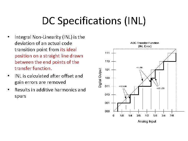
DC Specifications (INL) • Integral Non-Linearity (INL) is the deviation of an actual code transition point from its ideal position on a straight line drawn between the end points of the transfer function. • INL is calculated after offset and gain errors are removed • Results in additive harmonics and spurs

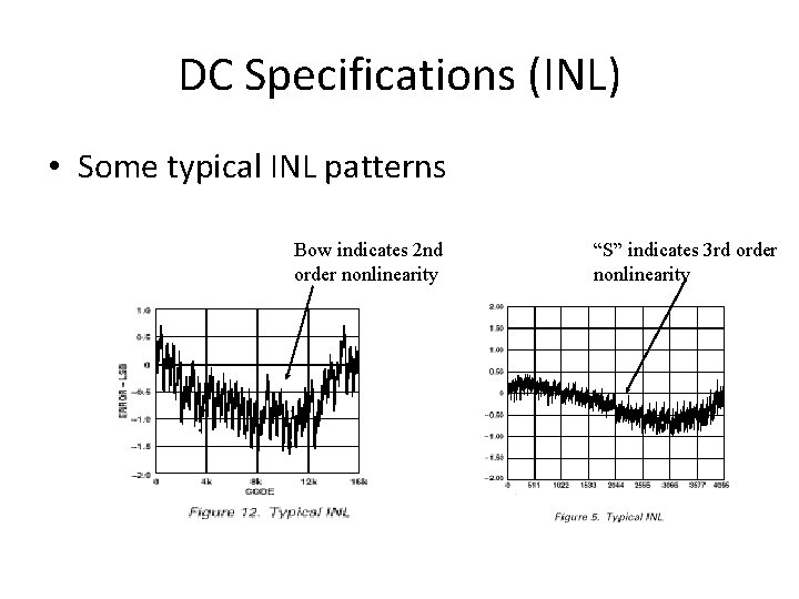
DC Specifications (INL) • Some typical INL patterns Bow indicates 2 nd order nonlinearity “S” indicates 3 rd order nonlinearity

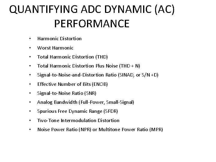
QUANTIFYING ADC DYNAMIC (AC) PERFORMANCE • Harmonic Distortion • Worst Harmonic • Total Harmonic Distortion (THD) • Total Harmonic Distortion Plus Noise (THD + N) • Signal-to-Noise-and-Distortion Ratio (SINAD, or S/N +D) • Effective Number of Bits (ENOB) • Signal-to-Noise Ratio (SNR) • Analog Bandwidth (Full-Power, Small-Signal) • Spurious Free Dynamic Range (SFDR) • Two-Tone Intermodulation Distortion • Noise Power Ratio (NPR) or Multitone Power Ratio (MPR)

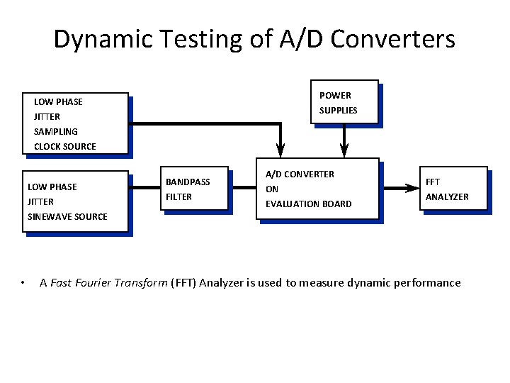
Dynamic Testing of A/D Converters POWER LOW PHASE SUPPLIES JITTER SAMPLING CLOCK SOURCE LOW PHASE JITTER SINEWAVE SOURCE • BANDPASS FILTER A/D CONVERTER ON EVALUATION BOARD FFT ANALYZER A Fast Fourier Transform (FFT) Analyzer is used to measure dynamic performance

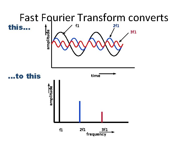
Fast Fourier Transform converts f 1 2 f 1 3 f 1 amplitude this… . . . to this amplitude time f 1 2 f 1 3 f 1 frequency

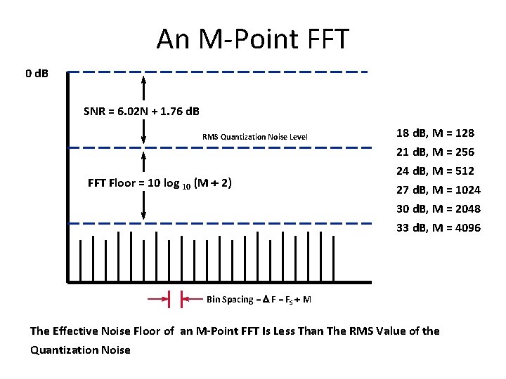
An M-Point FFT 0 d. B SNR = 6. 02 N + 1. 76 d. B RMS Quantization Noise Level FFT Floor = 10 log 10 (M ¸ 2) 18 d. B, M = 128 21 d. B, M = 256 24 d. B, M = 512 27 d. B, M = 1024 30 d. B, M = 2048 33 d. B, M = 4096 Bin Spacing = D F = FS ¸ M The Effective Noise Floor of an M-Point FFT Is Less Than The RMS Value of the Quantization Noise

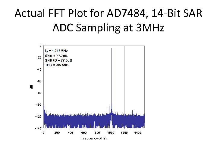
Actual FFT Plot for AD 7484, 14 -Bit SAR ADC Sampling at 3 MHz

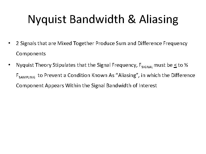
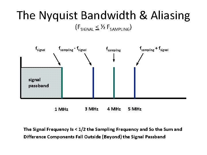
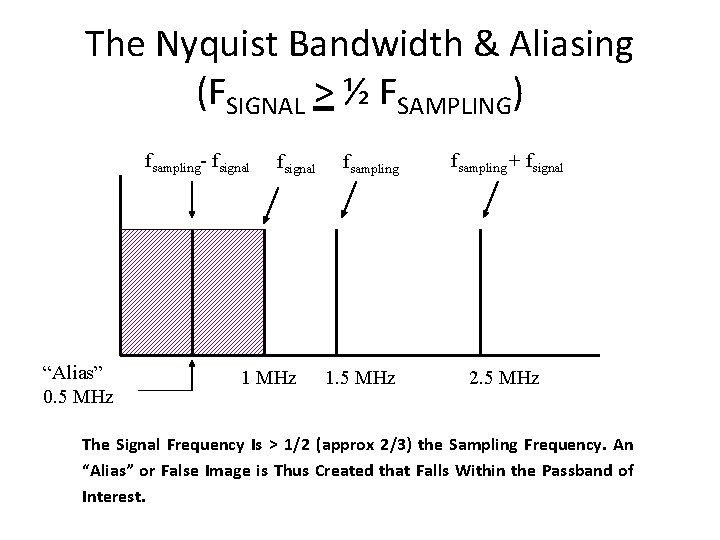
Nyquist Bandwidth & Aliasing • 2 Signals that are Mixed Together Produce Sum and Difference Frequency Components • Nyquist Theory Stipulates that the Signal Frequency, FSIGNAL must be < to ½ FSAMPLING to Prevent a Condition Known As “Aliasing”, in which the Difference Component Appears Within the Signal Bandwidth of Interest

The Nyquist Bandwidth & Aliasing (FSIGNAL < ½ FSAMPLING) fsignal fsampling - fsignal fsampling + fsignal passband 1 MHz 3 MHz 4 MHz 5 MHz The Signal Frequency Is < 1/2 the Sampling Frequency and So the Sum and Difference Components Fall Outside (Beyond) the Signal Passband

The Nyquist Bandwidth & Aliasing (FSIGNAL > ½ FSAMPLING) fsampling- fsignal “Alias” 0. 5 MHz fsignal 1 MHz fsampling 1. 5 MHz fsampling + fsignal 2. 5 MHz The Signal Frequency Is > 1/2 (approx 2/3) the Sampling Frequency. An “Alias” or False Image is Thus Created that Falls Within the Passband of Interest.

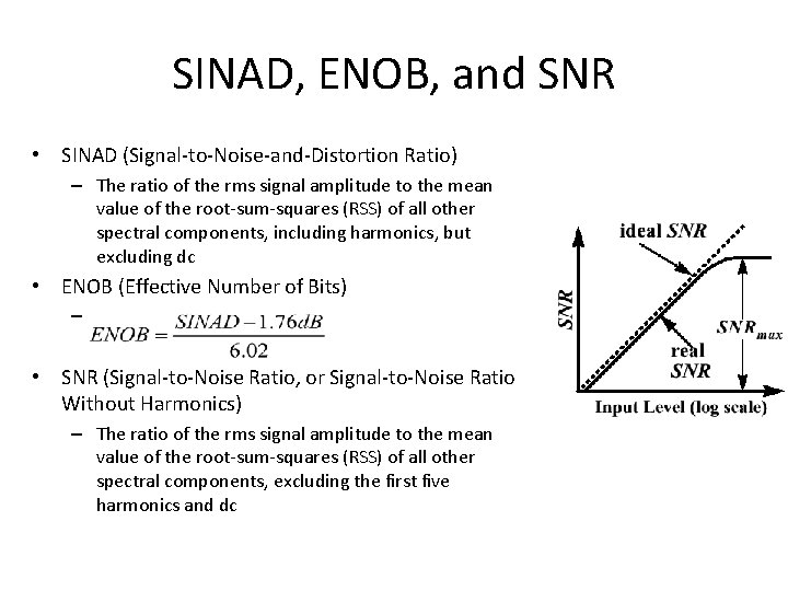
SINAD, ENOB, and SNR • SINAD (Signal-to-Noise-and-Distortion Ratio) – The ratio of the rms signal amplitude to the mean value of the root-sum-squares (RSS) of all other spectral components, including harmonics, but excluding dc • ENOB (Effective Number of Bits) – • SNR (Signal-to-Noise Ratio, or Signal-to-Noise Ratio Without Harmonics) – The ratio of the rms signal amplitude to the mean value of the root-sum-squares (RSS) of all other spectral components, excluding the first five harmonics and dc

ADC LARGE SIGNAL (OR FULL POWER) BANDWIDTH • Full-power bandwidth is defined as the input frequency where the fundamental in an FFT of the output, rolls off to its 3 d. B point • ADC’s SHA generally determines the FPBW – FPBW often limited by slew rate of the internal circuitry. – May not be compatible with the converter’s maximum operating rate • Ideally f. FPBW >> fs / 2 • Many High Speed Converters have f. FPBW < fs / 2 – Use as a “prerequisite” specification for comparing ADC’s IF undersampling capabilities. But need to consider distortion as well.

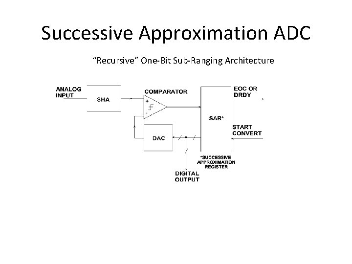
Successive Approximation ADC “Recursive” One-Bit Sub-Ranging Architecture

Successive Approximation ADC

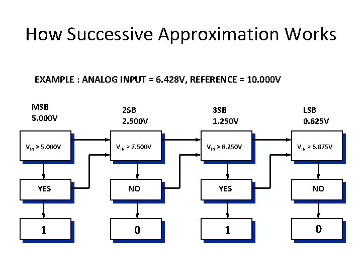
How a Successive Approximation A/D Converter Works • Rising/Falling Edge of Convert Start Pulse Resets Logic • Falling/Rising Edge Begins Conversion Process • Bit Comparisons Made on Each Clock Edge • Conversion Time Equals Number of Comparisons (Resolution) Times Clock Period • The Accuracy of Conversion Depends on the DAC Linearity and Comparator Noise

How Successive Approximation Works EXAMPLE : ANALOG INPUT = 6. 428 V, REFERENCE = 10. 000 V MSB 5. 000 V 2 SB 2. 500 V 3 SB 1. 250 V LSB 0. 625 V VIN > 5. 000 V VIN > 7. 500 V VIN > 6. 250 V VIN > 6. 875 V YES NO 0 1

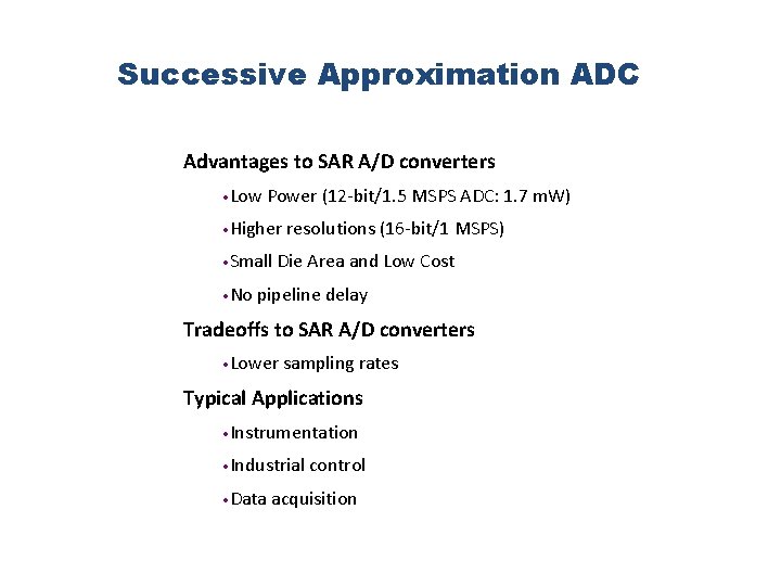
Successive Approximation ADC Advantages to SAR A/D converters • Low Power (12 -bit/1. 5 MSPS ADC: 1. 7 m. W) • Higher • Small • No resolutions (16 -bit/1 MSPS) Die Area and Low Cost pipeline delay Tradeoffs to SAR A/D converters • Lower sampling rates Typical Applications • Instrumentation • Industrial • Data control acquisition

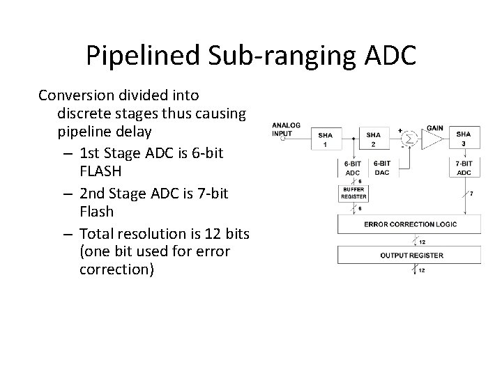
Pipelined Sub-ranging ADC Conversion divided into discrete stages thus causing pipeline delay – 1 st Stage ADC is 6 -bit FLASH – 2 nd Stage ADC is 7 -bit Flash – Total resolution is 12 bits (one bit used for error correction)

Pipelined Sub-ranging ADC

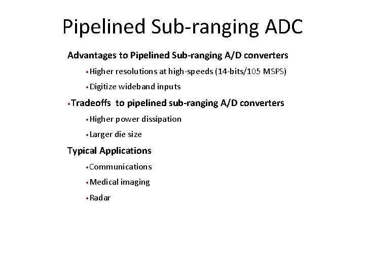
Pipelined Sub-ranging ADC Advantages to Pipelined Sub-ranging A/D converters • Higher resolutions at high-speeds (14 -bits/105 MSPS) • Digitize • Tradeoffs wideband inputs to pipelined sub-ranging A/D converters • Higher power dissipation • Larger die size Typical Applications • Communications • Medical • Radar imaging

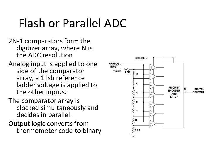
Flash or Parallel ADC 2 N-1 comparators form the digitizer array, where N is the ADC resolution Analog input is applied to one side of the comparator array, a 1 lsb reference ladder voltage is applied to the other inputs. The comparator array is clocked simultaneously and decides in parallel. Output logic converts from thermometer code to binary

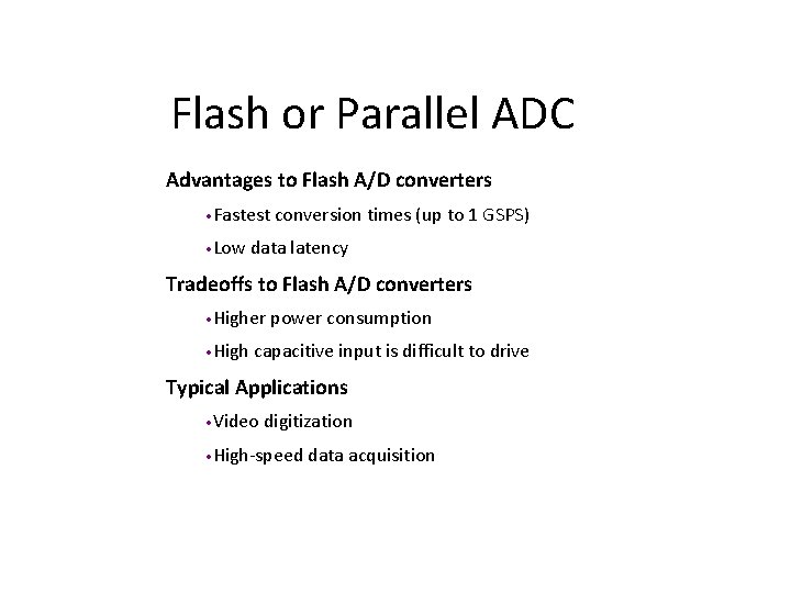
Flash or Parallel ADC Advantages to Flash A/D converters • Fastest • Low conversion times (up to 1 GSPS) data latency Tradeoffs to Flash A/D converters • Higher • High power consumption capacitive input is difficult to drive Typical Applications • Video digitization • High-speed data acquisition

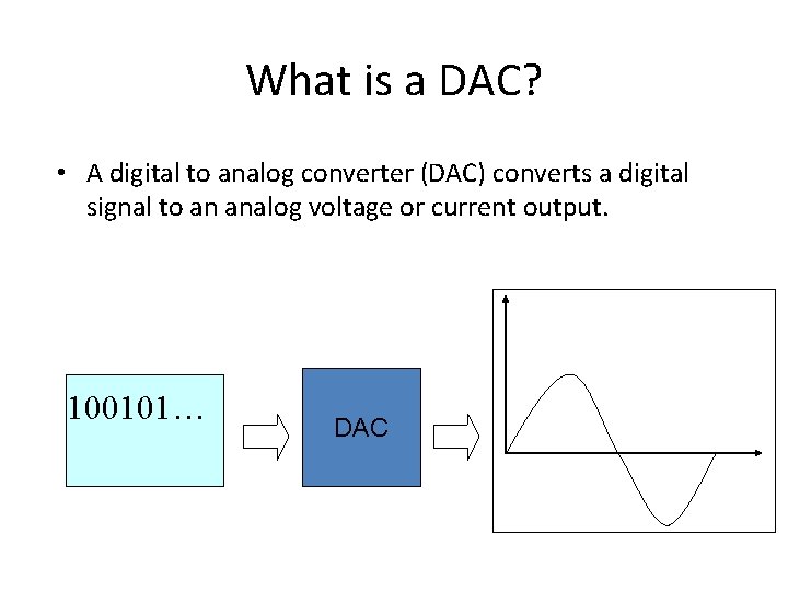
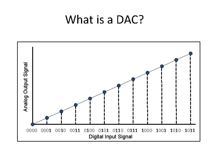
What is a DAC? • A digital to analog converter (DAC) converts a digital signal to an analog voltage or current output. 100101… DAC

Analog Output Signal What is a DAC? 0000 0001 0010 0011 0100 0101 0110 0111 1000 1001 1010 1011 Digital Input Signal

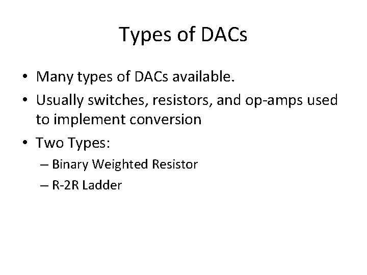
Types of DACs • Many types of DACs available. • Usually switches, resistors, and op-amps used to implement conversion • Two Types: – Binary Weighted Resistor – R-2 R Ladder

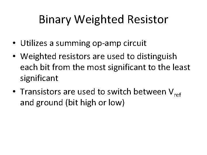
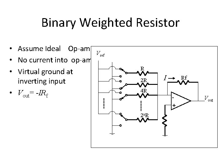
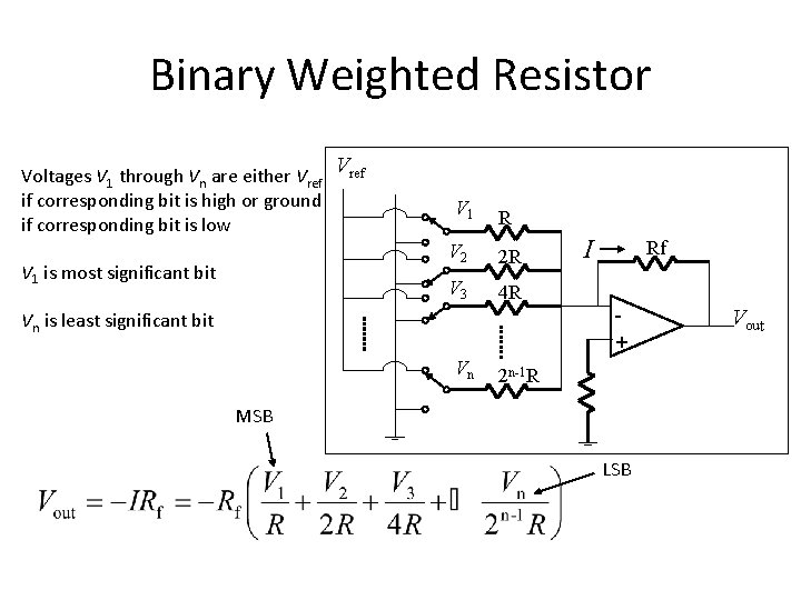
Binary Weighted Resistor • Utilizes a summing op-amp circuit • Weighted resistors are used to distinguish each bit from the most significant to the least significant • Transistors are used to switch between Vref and ground (bit high or low)

Binary Weighted Resistor • Assume Ideal Op-amp Vref • No current into op-amp • Virtual ground at inverting input • Vout= -IRf R 2 R I Rf 4 R + 2 n. R Vout

Binary Weighted Resistor Voltages V 1 through Vn are either Vref if corresponding bit is high or ground if corresponding bit is low V 1 is most significant bit Vref V 1 R V 2 2 R V 3 4 R Vn is least significant bit Vn I Rf + 2 n-1 R MSB LSB Vout

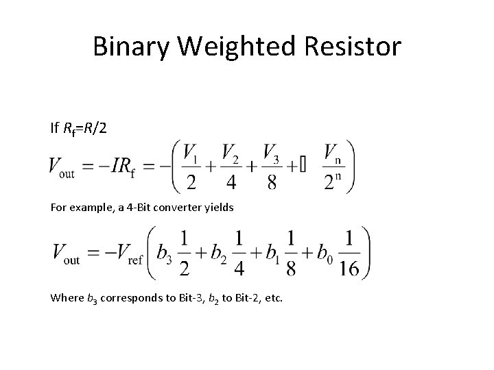
Binary Weighted Resistor If Rf=R/2 For example, a 4 -Bit converter yields Where b 3 corresponds to Bit-3, b 2 to Bit-2, etc.

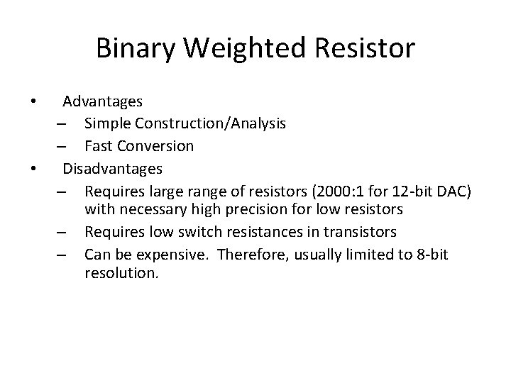
Binary Weighted Resistor • • Advantages – Simple Construction/Analysis – Fast Conversion Disadvantages – Requires large range of resistors (2000: 1 for 12 -bit DAC) with necessary high precision for low resistors – Requires low switch resistances in transistors – Can be expensive. Therefore, usually limited to 8 -bit resolution.

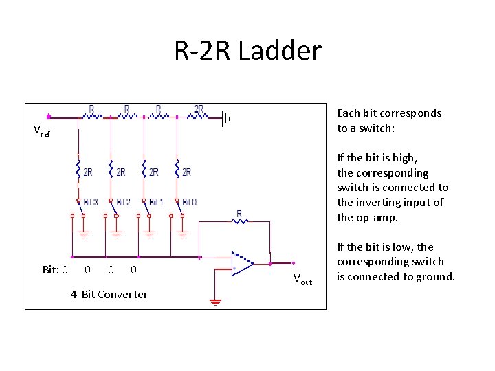
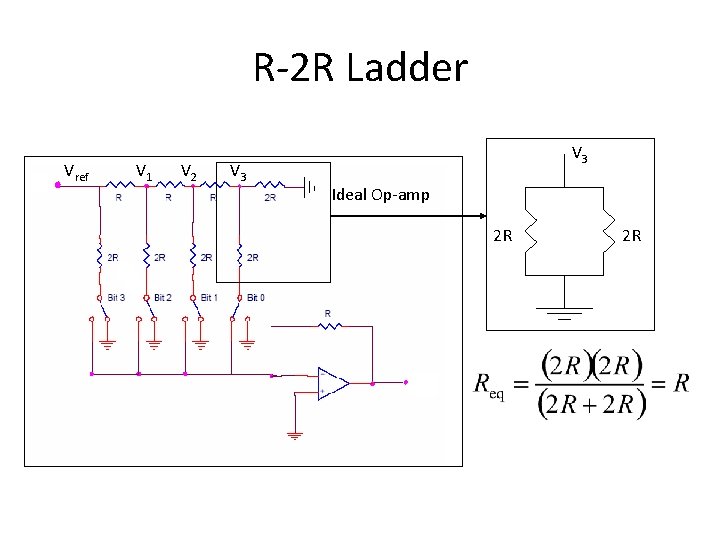
R-2 R Ladder Each bit corresponds to a switch: Vref If the bit is high, the corresponding switch is connected to the inverting input of the op-amp. Bit: 0 0 4 -Bit Converter Vout If the bit is low, the corresponding switch is connected to ground.

R-2 R Ladder Vref V 1 V 2 V 3 Ideal Op-amp 2 R 2 R

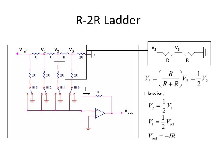
R-2 R Ladder Vref V 1 V 2 V 3 R I Likewise, Vout R

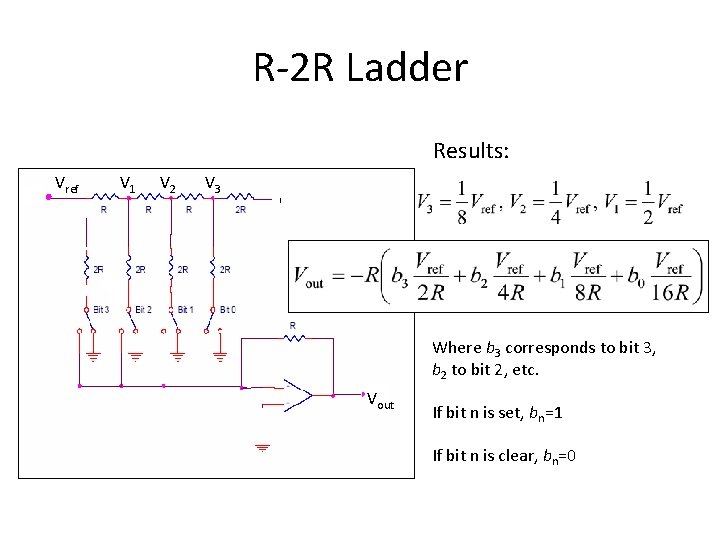
R-2 R Ladder Results: Vref V 1 V 2 V 3 Where b 3 corresponds to bit 3, b 2 to bit 2, etc. Vout If bit n is set, bn=1 If bit n is clear, bn=0

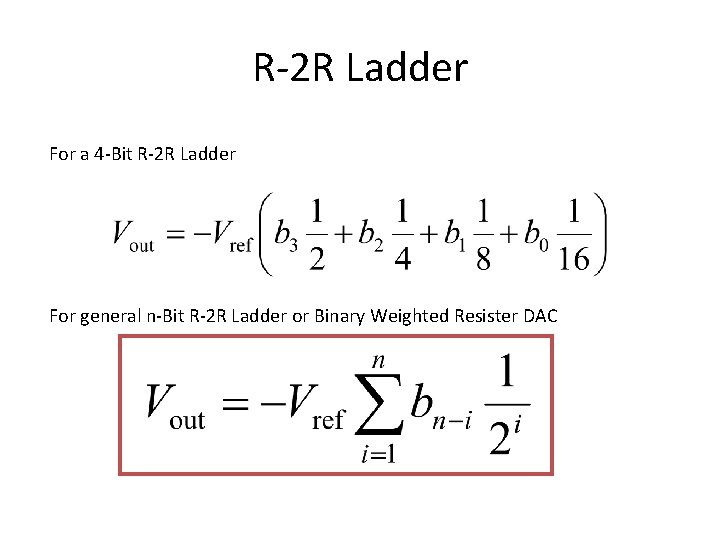
R-2 R Ladder For a 4 -Bit R-2 R Ladder For general n-Bit R-2 R Ladder or Binary Weighted Resister DAC

R-2 R Ladder • Advantages – Only two resistor values (R and 2 R) – Does not require high precision resistors • Disadvantage – Lower conversion speed than binary weighted DAC

Specifications of DACs • • • Resolution Speed Linearity Settling Time Reference Voltages Errors

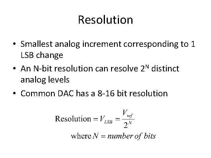
Resolution • Smallest analog increment corresponding to 1 LSB change • An N-bit resolution can resolve 2 N distinct analog levels • Common DAC has a 8 -16 bit resolution

Speed • Rate of conversion of a single digital input to its analog equivalent • Conversion rate depends on – clock speed of input signal – settling time of converter • When the input changes rapidly, the DAC conversion speed must be high.

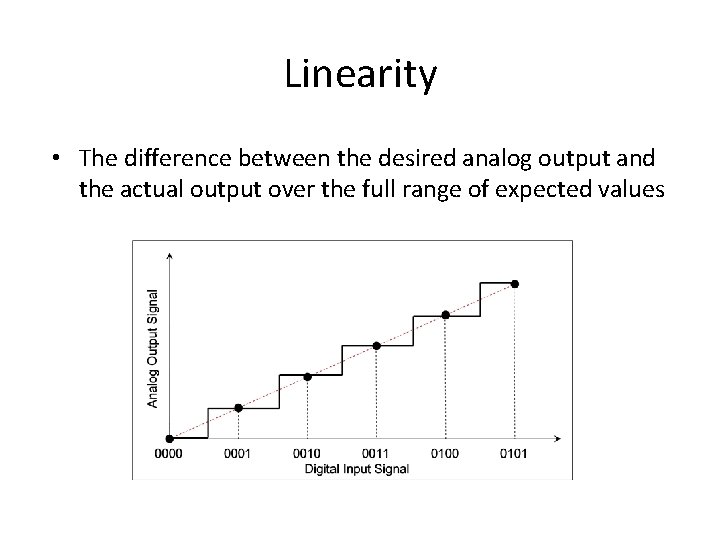
Linearity • The difference between the desired analog output and the actual output over the full range of expected values

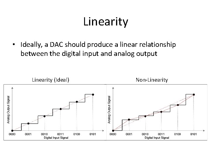
Linearity • Ideally, a DAC should produce a linear relationship between the digital input and analog output Linearity (Ideal) Non-Linearity

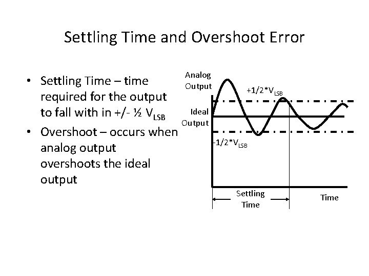
Settling Time • Time required for the output signal to settle within +/- ½ LSB of its final value after a given change in input scale • Limited by slew rate of output amplifier • Ideally, an instantaneous change in analog voltage would occur when a new binary word enters into DAC

Reference Voltages • Used to determine how each digital input will be assigned to each voltage division • Types: – Non-multiplier DAC: Vref is fixed – Multiplier DAC: Vref provided by external source

Types of Errors Associated with DACs • • Gain Offset Full Scale Resolution Non-Linearity Non-Monotonic Settling Time and Overshoot

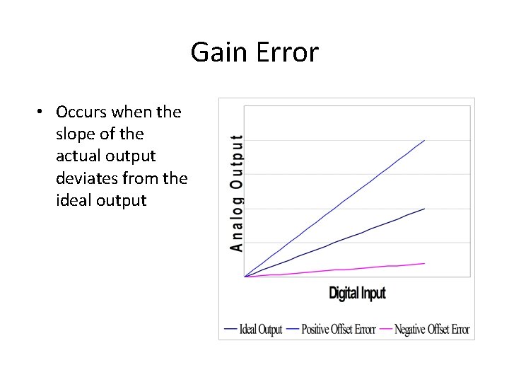
Gain Error • Occurs when the slope of the actual output deviates from the ideal output

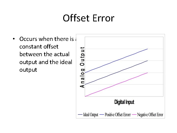
Offset Error • Occurs when there is a constant offset between the actual output and the ideal output

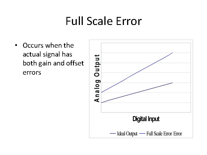
Full Scale Error • Occurs when the actual signal has both gain and offset errors

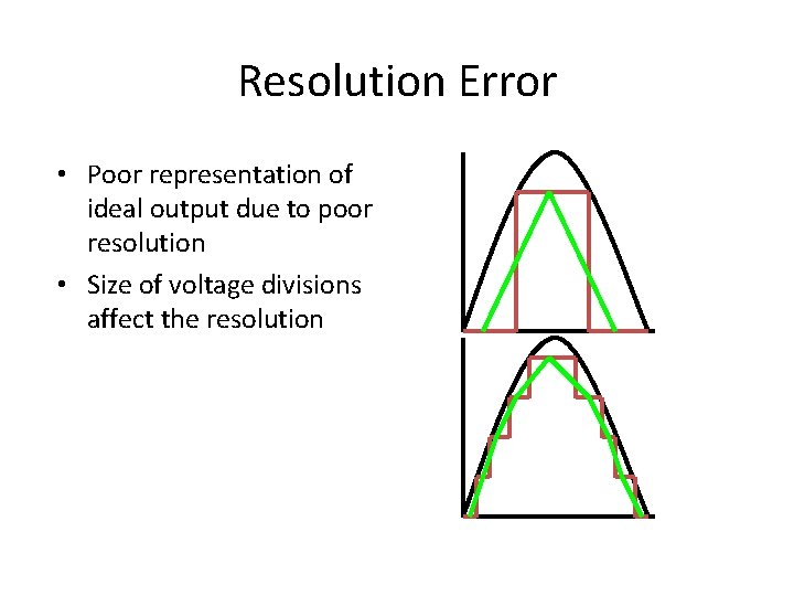
Resolution Error • Poor representation of ideal output due to poor resolution • Size of voltage divisions affect the resolution

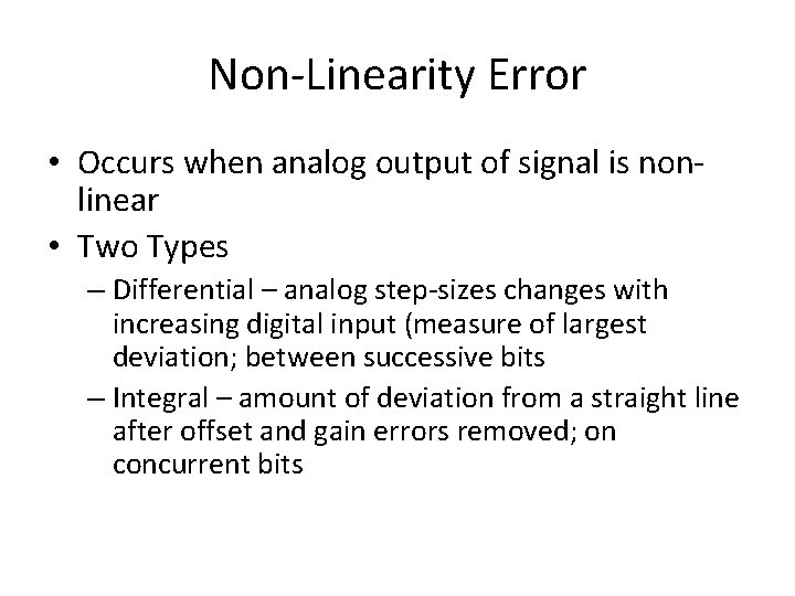
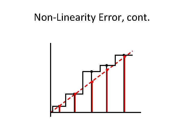
Non-Linearity Error • Occurs when analog output of signal is nonlinear • Two Types – Differential – analog step-sizes changes with increasing digital input (measure of largest deviation; between successive bits – Integral – amount of deviation from a straight line after offset and gain errors removed; on concurrent bits

Non-Linearity Error, cont.

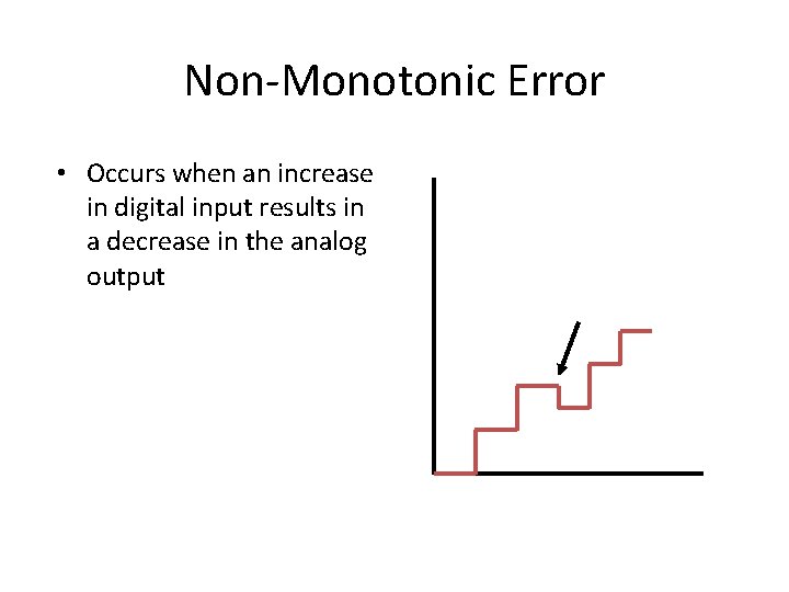
Non-Monotonic Error • Occurs when an increase in digital input results in a decrease in the analog output

Settling Time and Overshoot Error Analog • Settling Time – time Output +1/2*VLSB required for the output Ideal to fall with in +/- ½ VLSB Output • Overshoot – occurs when -1/2*VLSB analog output overshoots the ideal output Settling Time

Exponential and logarithm

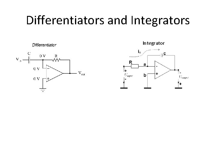
Differentiators and Integrators Integrator