Mixed Tools for Market Analysis and Their Applications

Mixed Tools for Market Analysis and Their Applications Boris Goldengorin LATNA – Laboratory of Algorithms and Technologies for Network Analysis Higher School of Economics, Moscow, Russian Federation bgoldengorin@hse. ru Joint work with M. Batsyn, V. Kalyagin, A. Kocheturov, P. M. Pardalos, A. Vizgunov

Dedicated to Boris Mirkin Birthday • Professor, Department of Applied Mathematics, Higher School of Economics, Moscow RF • • • - clustering - decision making - mathematical classification - evolutionary trees - data and text interpretation • Citation indices • • All Citations 3865 h-index 28 i 10 -index 50 2

Mirkin visit me in Alma-Ata, Kazakhstan in 1981 The USSR Workshop on Statistical and Discrete Analysis of Non. Numerical Information, Expert’s Estimations and Discrete Optimization. Abstracts. Moscow-Alma-Ata, VINITI AN SSSR, 1981, pp. 356 (in Russian) 3

Abstract • Efficient daily trading impose aggregation of positions correlated to each other by one of trader’s criteria. The positions aggregation is one of possible ways to increase the online trader’s capacity. • In this talk we analyse the well known minimum spanning tree (forest) approach used for the market graphs analysis and combine this approach with less known pseudo-Boolean approach based on the p-median problem. • We illustrate our mixed tools (spanning p-forest combined with pstars) by application them to different sources of data including market graphs and cell formation in group technology. 4

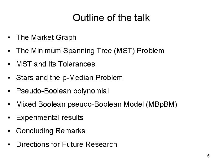
Outline of the talk • The Market Graph • The Minimum Spanning Tree (MST) Problem • MST and Its Tolerances • Stars and the p-Median Problem • Pseudo-Boolean polynomial • Mixed Boolean pseudo-Boolean Model (MBp. BM) • Experimental results • Concluding Remarks • Directions for Future Research 5

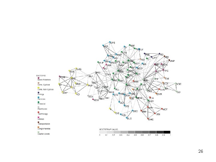
Market Graph • Vertices are stocks, and an edge connects two stocks if the correlation between their price fluctuations over a certain period is greater than a specified threshold • ~6000 vertices (stocks) 6

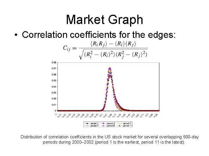
Market Graph • Correlation coefficients for the edges: Distribution of correlation coefficients in the US stock market for several overlapping 500 -day periods during 2000– 2002 (period 1 is the earliest, period 11 is the latest).

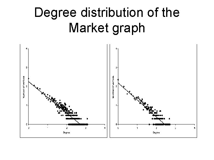
Market Graph • Market graph (all the considered instances for different correlation thresholds) follows the power-law model • Using the combination of heuristic and exact algorithms, the exact solution of the maximum clique problem was found (Boginski, Butenko & Pardalos, 2005)

Degree distribution of the Market graph

Finding Cliques in the Market graph • Using the IP formulation of the maximum clique problem to find the exact solution:

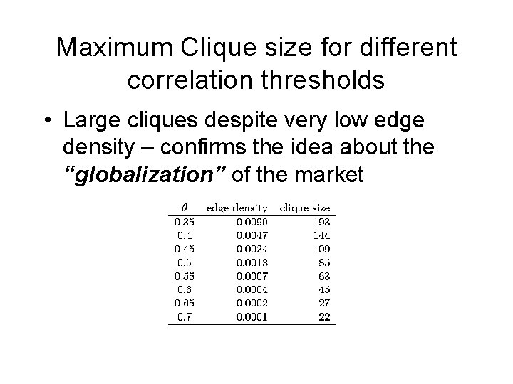
Maximum Clique size for different correlation thresholds • Large cliques despite very low edge density – confirms the idea about the “globalization” of the market

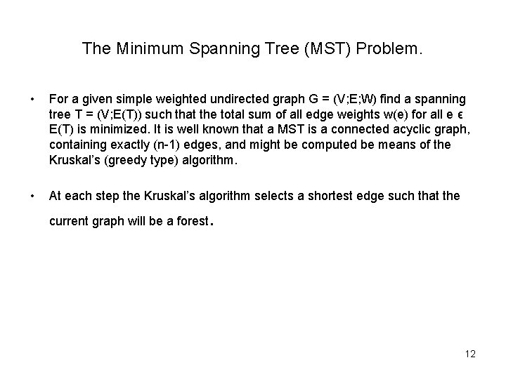
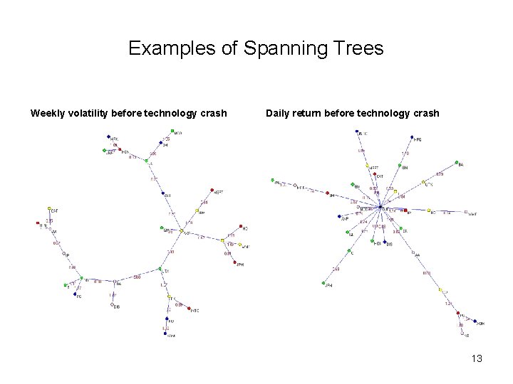
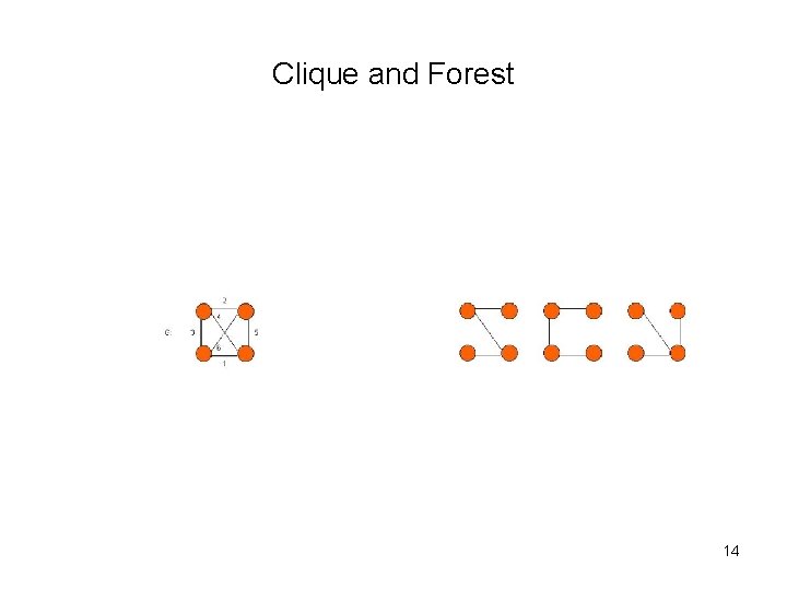
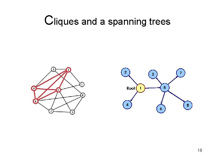
The Minimum Spanning Tree (MST) Problem. • For a given simple weighted undirected graph G = (V; E; W) find a spanning tree T = (V; E(T)) such that the total sum of all edge weights w(e) for all e ϵ E(T) is minimized. It is well known that a MST is a connected acyclic graph, containing exactly (n-1) edges, and might be computed be means of the Kruskal’s (greedy type) algorithm. • At each step the Kruskal’s algorithm selects a shortest edge such that the current graph will be a forest . 12

Examples of Spanning Trees Weekly volatility before technology crash Daily return before technology crash 13

Clique and Forest 14

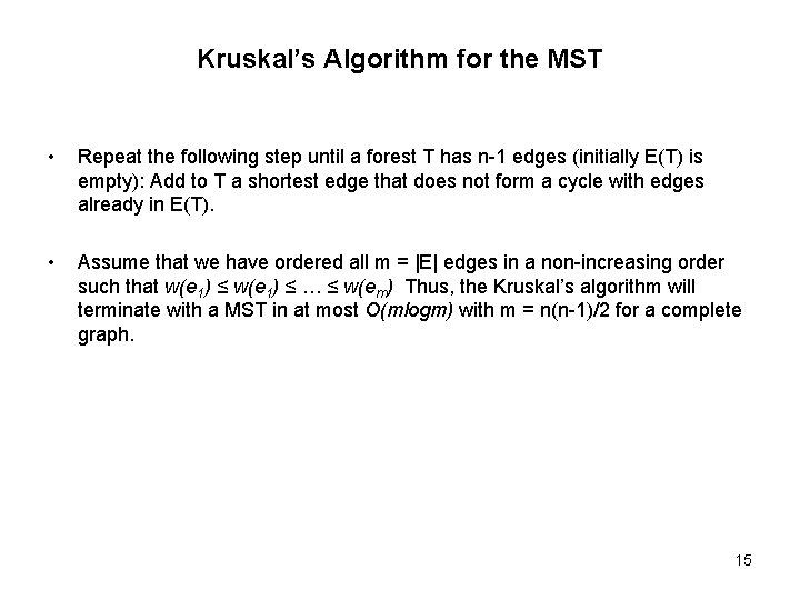
Kruskal’s Algorithm for the MST • Repeat the following step until a forest T has n-1 edges (initially E(T) is empty): Add to T a shortest edge that does not form a cycle with edges already in E(T). • Assume that we have ordered all m = |E| edges in a non-increasing order such that w(e 1) ≤ … ≤ w(em) Thus, the Kruskal’s algorithm will terminate with a MST in at most O(mlogm) with m = n(n-1)/2 for a complete graph. 15

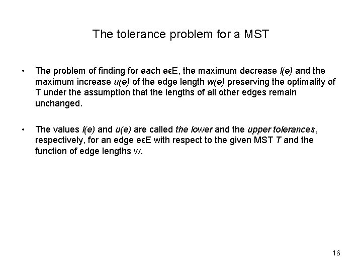
The tolerance problem for a MST • The problem of finding for each eϵE, the maximum decrease l(e) and the maximum increase u(e) of the edge length w(e) preserving the optimality of T under the assumption that the lengths of all other edges remain unchanged. • The values l(e) and u(e) are called the lower and the upper tolerances, respectively, for an edge eϵE with respect to the given MST T and the function of edge lengths w. 16

An optimal MST and Its Tolerances in O(mlogm) time In the following portion we show that a MST together with all its upper and lower tolerances can be computed in O(mlogm) time by a tiny modification of the Kruskal’s algorithm. Let us recall that by adding a single edge y not in T to the chosen spanning subtree S(T) we create a unique cycle C = {e 1; e 2, …, ek, y} where the tail of y is the head of ek and the head of y is the tail of e 1 or vice versa. 17

Cliques and a spanning trees 18

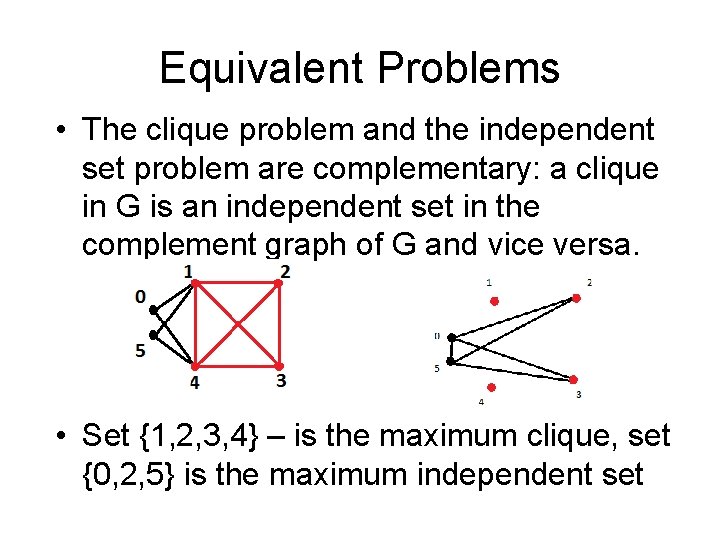
Equivalent Problems • The clique problem and the independent set problem are complementary: a clique in G is an independent set in the complement graph of G and vice versa. • Set {1, 2, 3, 4} – is the maximum clique, set {0, 2, 5} is the maximum independent set

Market Graph • Vertices are stocks, and an edge connects two stocks if the correlation between their price fluctuations over a certain period is greater than a specified threshold • ~6000 vertices (stocks) 20

Market Graph • Correlation coefficients for the edges: Distribution of correlation coefficients in the US stock market for several overlapping 500 -day periods during 2000– 2002 (period 1 is the earliest, period 11 is the latest).

Market Graph • Market graph (all the considered instances for different correlation thresholds) follows the power-law model • Using the combination of heuristic and exact algorithms, the exact solution of the maximum clique problem was found (Boginski, Butenko & Pardalos, 2005)

Degree distribution of the Market graph

Finding Cliques in the Market graph • Using the IP formulation of the maximum clique problem to find the exact solution:

Maximum Clique size for different correlation thresholds • Large cliques despite very low edge density – confirms the idea about the “globalization” of the market

26

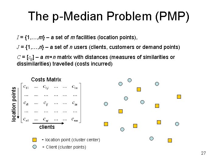
The p-Median Problem (PMP) I = {1, …, m} – a set of m facilities (location points), J = {1, …, n} – a set of n users (clients, customers or demand points) C = [cij] – a m×n matrix with distances (measures of similarities or dissimilarities) travelled (costs incurred) location points Costs Matrix clients - location point (cluster center) - Client (cluster points) 27

The PMP: combinatorial formulation complexity The p-Median Problem (PMP) consists of determining p locations (the median points) such that 1 ≤ p ≤ m and the sum of distances (or transportation costs) over all clients is minimal. 1 m p - opened facility - location point - client p = 3 28

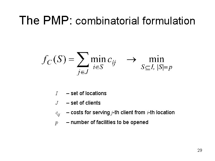
The PMP: combinatorial formulation I – set of locations J – set of clients cij – costs for serving j-th client from i-th location p – number of facilities to be opened 29

The PMP: Applications • Facilty location • Cluster analysis • Quantitative psychology • Telecommunications industry • Sales force territories design • Political and administrative districting • Optimal diversity management (assortment problems) • Cell formation in group technology (flexible manufacturing systems) • Vehicle routing • Topological design of computer and communication networks 30

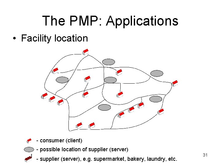
The PMP: Applications • Facility location - consumer (client) - possible location of supplier (server) - supplier (server), e. g. supermarket, bakery, laundry, etc. 31

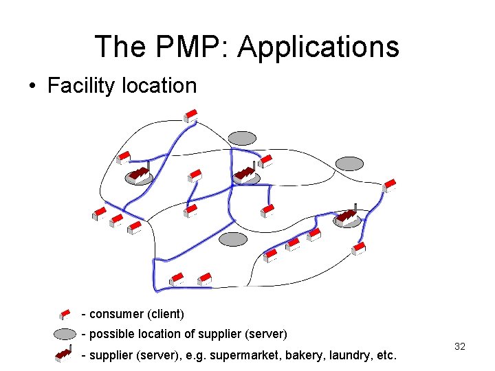
The PMP: Applications • Facility location - consumer (client) - possible location of supplier (server) - supplier (server), e. g. supermarket, bakery, laundry, etc. 32

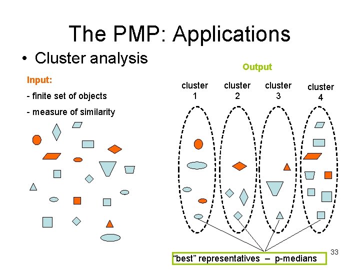
The PMP: Applications • Cluster analysis Input: - finite set of objects Output cluster 1 cluster 2 cluster 3 cluster 4 - measure of similarity “best” representatives – p-medians 33

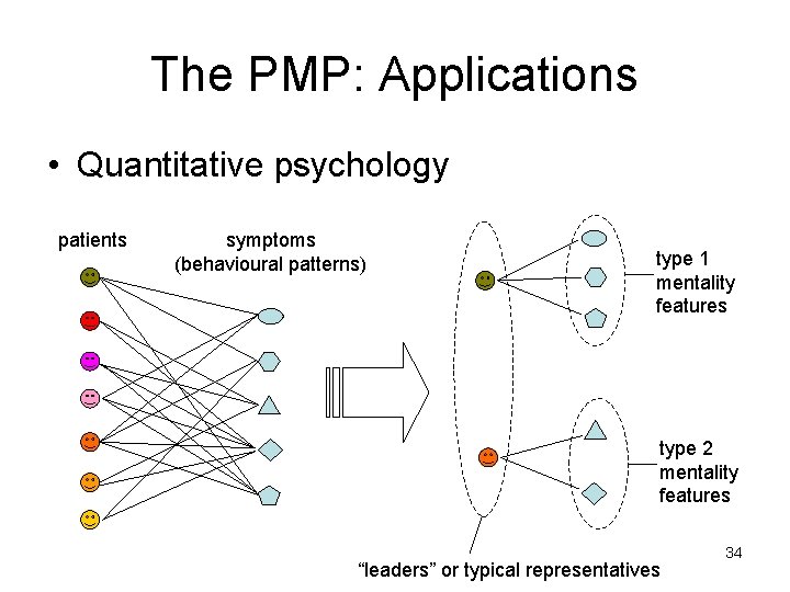
The PMP: Applications • Quantitative psychology patients symptoms (behavioural patterns) type 1 mentality features type 2 mentality features “leaders” or typical representatives 34

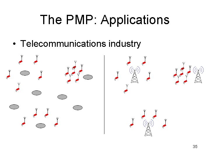
The PMP: Applications • Telecommunications industry 35

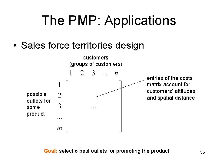
The PMP: Applications • Sales force territories design customers (groups of customers) possible outlets for some product entries of the costs matrix account for customers’ attitudes and spatial distance Goal: select p best outlets for promoting the product 36

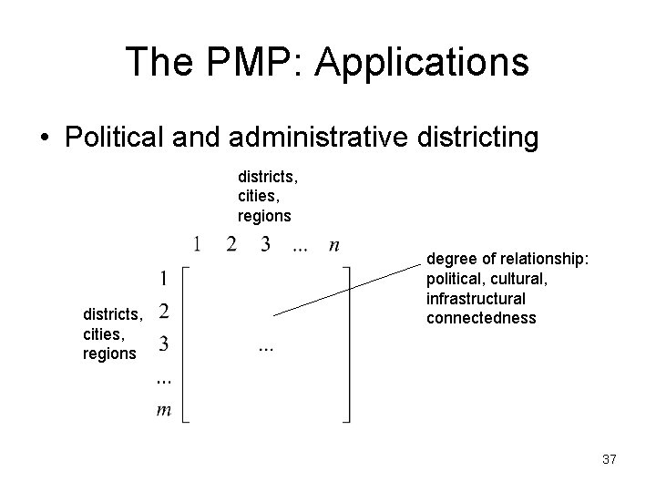
The PMP: Applications • Political and administrative districting districts, cities, regions degree of relationship: political, cultural, infrastructural connectedness 37

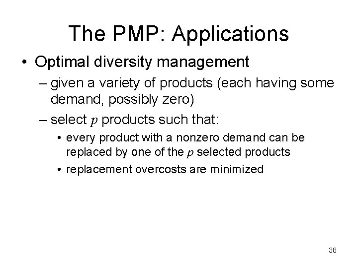
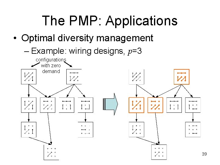
The PMP: Applications • Optimal diversity management – given a variety of products (each having some demand, possibly zero) – select p products such that: • every product with a nonzero demand can be replaced by one of the p selected products • replacement overcosts are minimized 38

The PMP: Applications • Optimal diversity management – Example: wiring designs, p=3 configurations with zero demand 39

The PMP: Applications • Cell formation in group technology functional layout - machines - products routes cellular layout see also video at http: //www. youtube. com/watch? v=q_m 0_b. VAJb. A 40

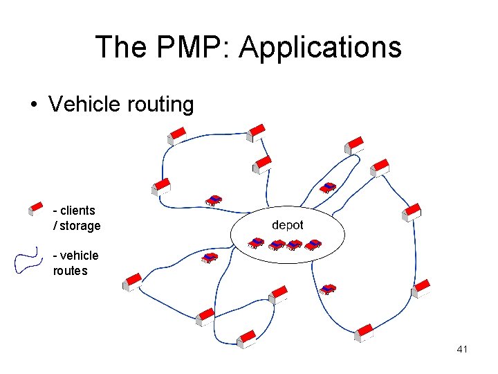
The PMP: Applications • Vehicle routing - clients / storage - vehicle routes 41

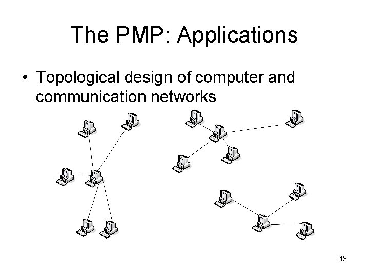
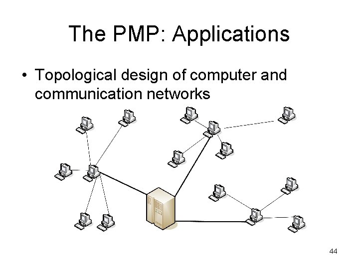
The PMP: Applications • Topological design of computer and communication networks 42

The PMP: Applications • Topological design of computer and communication networks 43

The PMP: Applications • Topological design of computer and communication networks 44

Publications, more than 500 Goldengorin et al, 2011, 2012 Elloumi, 2010; Brusco and K¨ohn, 2008; Belenky, 2008; Church, 2003; 2008; Avella et al, 2007; Beltran et al, 2006; Reese, 2006 (Overview, NETWORKS) Re. Velle and Swain, 1970; Senne et al, 2005. 45

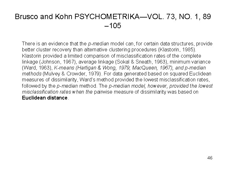
Brusco and Kohn PSYCHOMETRIKA—VOL. 73, NO. 1, 89 – 105 There is an evidence that the p-median model can, for certain data structures, provide better cluster recovery than alternative clustering procedures (Klastorin, 1985). Klastorin provided a limited comparison of misclassification rates of the complete linkage (Johnson, 1967), average linkage (Sokal & Sneath, 1963), minimum variance (Ward, 1963), K-means (Hartigan & Wong, 1979; Mac. Queen, 1967), and p-median methods (Mulvey & Crowder, 1979). For data generated based on squared Euclidean measures of dissimilarity, Ward’s method provided the lowest misclassification rates, followed by the p-median method. The p-median model, however, provided the lowest misclassification rates when the pairwise measure of dissimilarity was based on Euclidean distance. 46

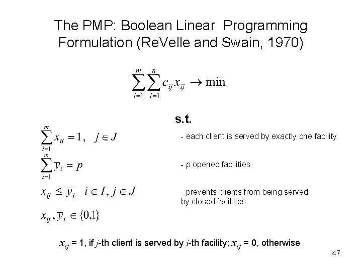
The PMP: Boolean Linear Programming Formulation (Re. Velle and Swain, 1970) s. t. - each client is served by exactly one facility - p opened facilities - prevents clients from being served by closed facilities xij = 1, if j-th client is served by i-th facility; xij = 0, otherwise 47

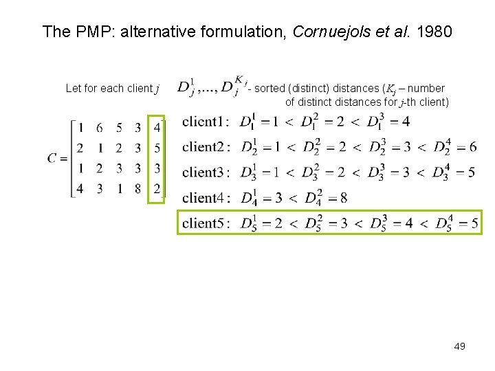
The PMP: alternative formulation, Cornuejols et al. 1980 Let for each client j - sorted (distinct) distances (Kj – number of distinct distances for j-th client) 48

The PMP: alternative formulation, Cornuejols et al. 1980 Let for each client j - sorted (distinct) distances (Kj – number of distinct distances for j-th client) 49

The PMP: alternative formulation, Cornuejols et al. 1980 Let for each client j - sorted (distinct) distances (Kj – number of distinct distances for j-th client) Decision variables S - set of opened plants 50

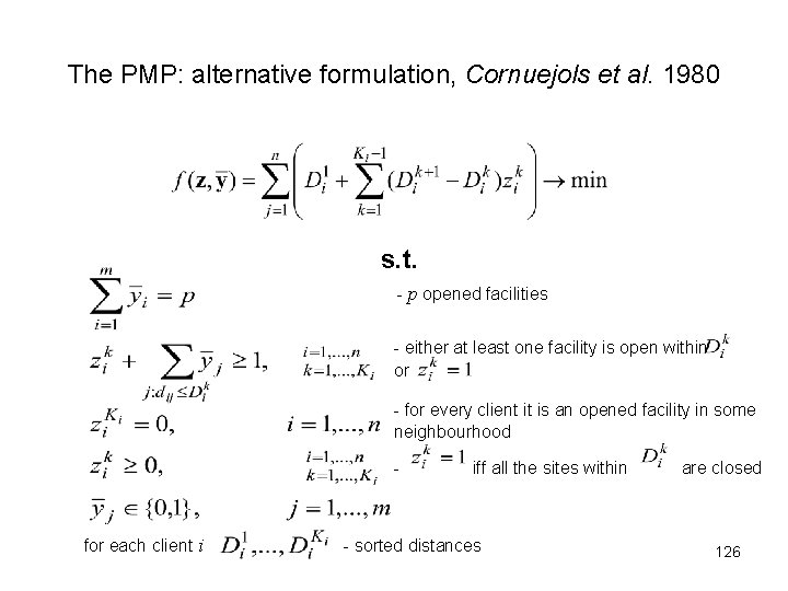
The PMP: alternative formulation, Cornuejols et al. 1980 s. t. - p opened facilities - either at least one facility is open within or - for every client it is an opened facility in some neighbourhood - iff all the sites within are closed for each client i - sorted distances 51

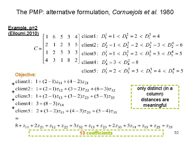
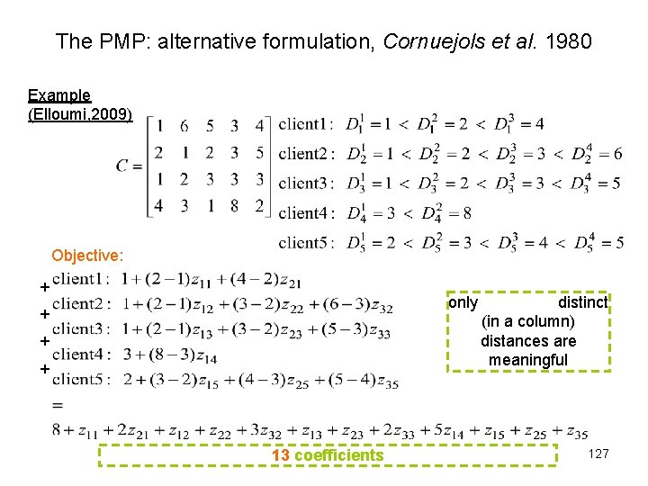
The PMP: alternative formulation, Cornuejols et al. 1980 Example, p=2 (Elloumi, 2010) Objective: + + only distinct (in a column) distances are meaningful 13 coefficients 52

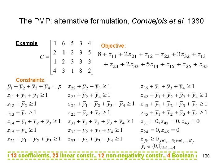
The PMP: alternative formulation, Cornuejols et al. 1980 Example Objective: Constraints: 13 coefficients, 23 linear constr. , 12 non-negativity constr. , 4 Boolean 53

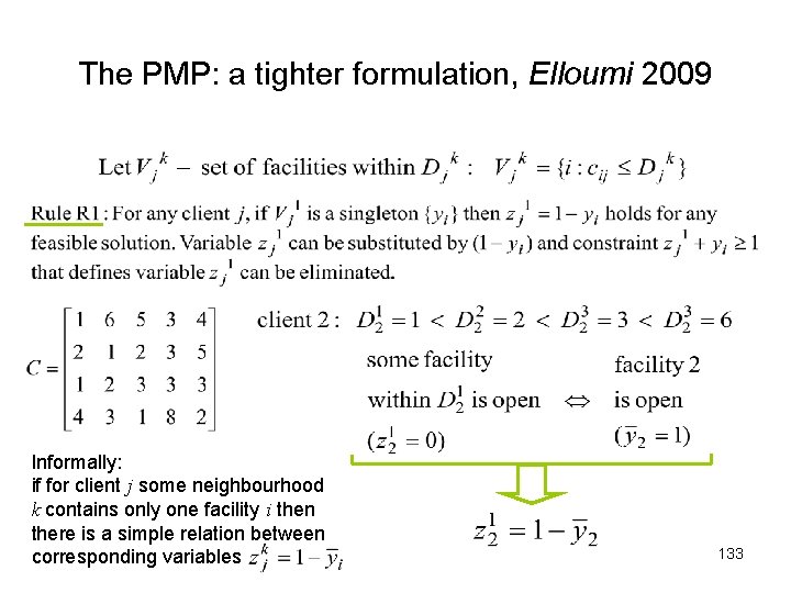
The p-Median Problem: a tighter formulation, Elloumi 2010 Informally: if for client j some neighbourhood k contains only one facility i then there is a simple relation between corresponding variables 54

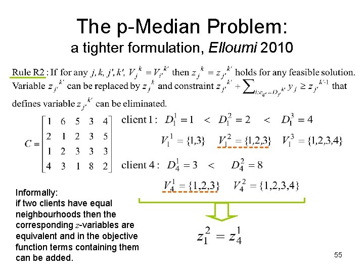
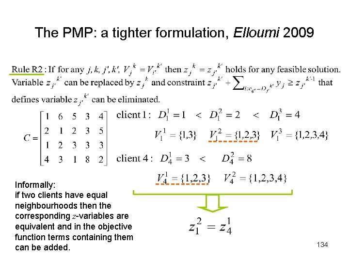
The p-Median Problem: a tighter formulation, Elloumi 2010 Informally: if two clients have equal neighbourhoods then the corresponding z-variables are equivalent and in the objective function terms containing them can be added. 55

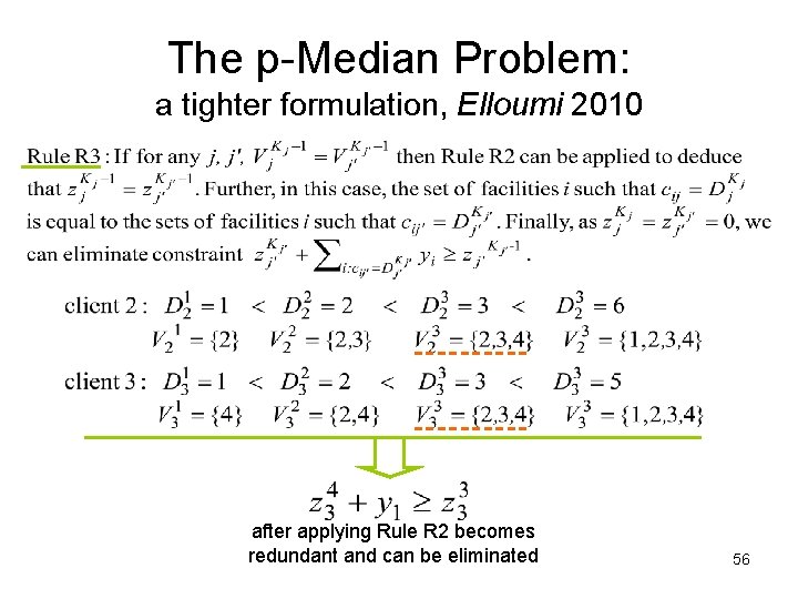
The p-Median Problem: a tighter formulation, Elloumi 2010 after applying Rule R 2 becomes redundant and can be eliminated 56

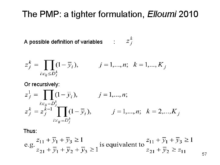
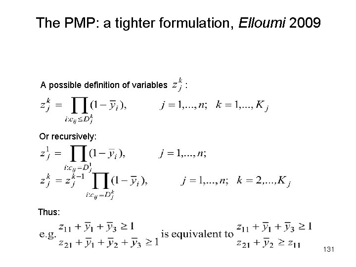
The PMP: a tighter formulation, Elloumi 2010 A possible definition of variables : Or recursively: Thus: 57

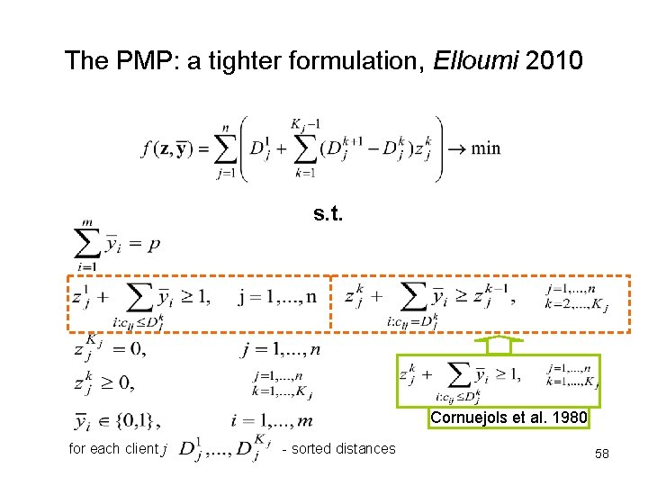
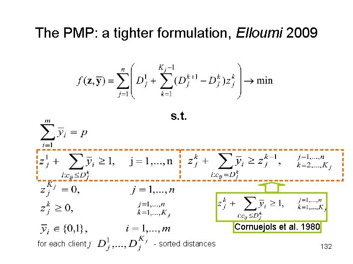
The PMP: a tighter formulation, Elloumi 2010 s. t. Cornuejols et al. 1980 for each client j - sorted distances 58

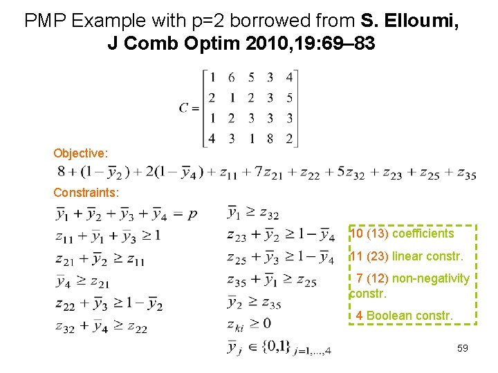
PMP Example with p=2 borrowed from S. Elloumi, J Comb Optim 2010, 19: 69– 83 Objective: Constraints: 10 (13) coefficients 11 (23) linear constr. 7 (12) non-negativity constr. 4 Boolean constr. 59

The PMP: pseudo-Boolean formulation (Historical remarks) • Hammer, 1968 for the Simple Plant Location Problem (SPLP) called also Uncapacitated Faciltiy Location Problem. His formulation contains both literals and their complements, but at the end of this paper Hammer has considered an inversion of literals; • Beresnev, 1971 for the SPLP applied to the so called standardization (unification) problem. He has changed the definition of decision variables, namely for an opened site a Boolean variable is equal to 0, and for a closed site a Boolean variable is equal to 1. This is exactly what is done by Cornuejols et al. 1980 and later on by Elloumi 2010 but as we will show by means of computational experiments with a larger number of decision variables and constraints. Beresnev’s formulation contains complements only for linear terms and all nonlinear terms are without complements. 60

The PMP and SPLP differ in the following details • SPLP involves fixed cost for location a facility at the given site, while the PMP does not; • Unlike the PMP, SPLP does not have a constraint on the number of opened facilities; • Typical SPLP formulations separate the set of potential facilities (sites location, cluster centers) from the set of demand points (clients); • In the PMP the sets of sites location and demand points are identical, i. e. I=J; • The SPLP with a constraint on the number of opened facilities is called either Capacitated SPLP or Generalized PMP. 61

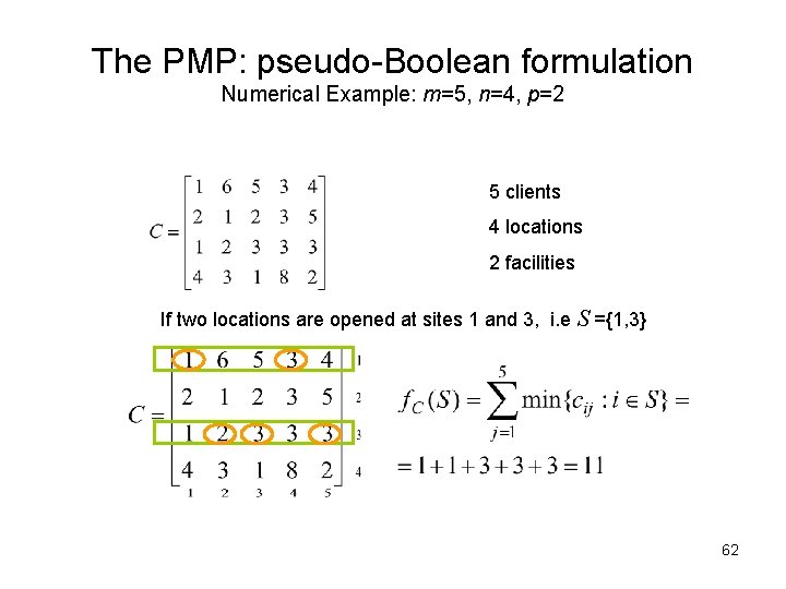
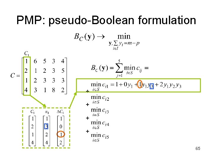
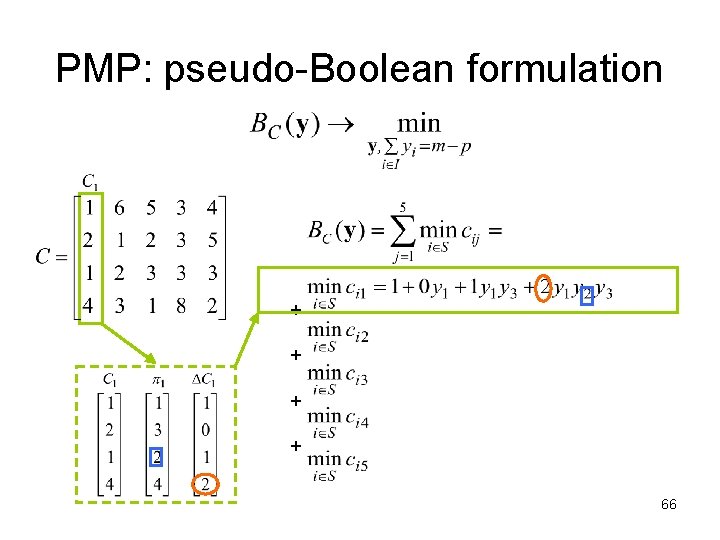
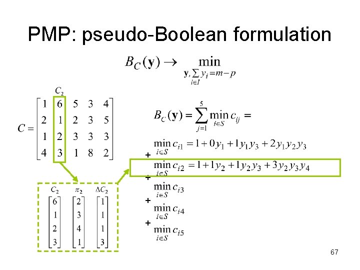
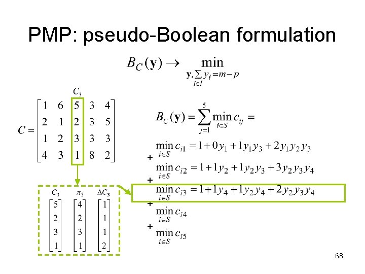
The PMP: pseudo-Boolean formulation Numerical Example: m=5, n=4, p=2 5 clients 4 locations 2 facilities If two locations are opened at sites 1 and 3, i. e S ={1, 3} 62

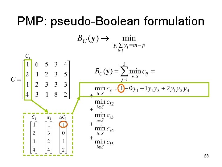
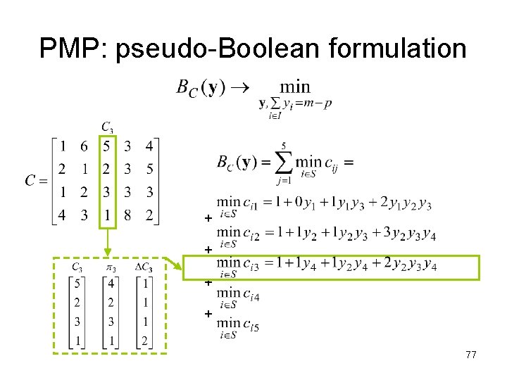
PMP: pseudo-Boolean formulation + + 63

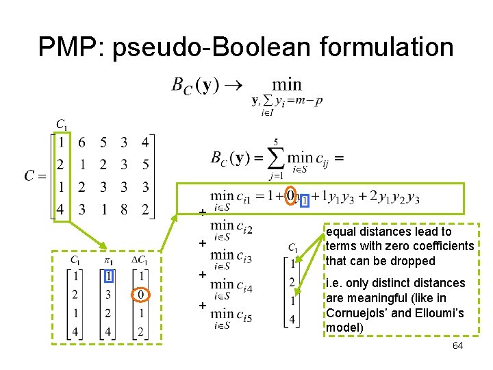
PMP: pseudo-Boolean formulation + + equal distances lead to terms with zero coefficients that can be dropped i. e. only distinct distances are meaningful (like in Cornuejols’ and Elloumi’s model) 64

PMP: pseudo-Boolean formulation + + 65

PMP: pseudo-Boolean formulation + + 66

PMP: pseudo-Boolean formulation + + 67

PMP: pseudo-Boolean formulation + + 68

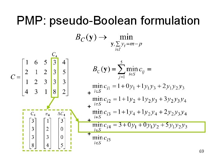
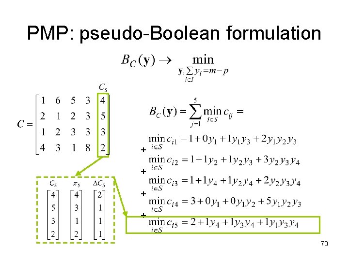
PMP: pseudo-Boolean formulation + + 69

PMP: pseudo-Boolean formulation + + 70

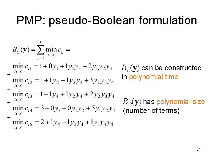
PMP: pseudo-Boolean formulation + + BC(y) can be constructed in polynomial time BC(y) has polynomial size (number of terms) 71

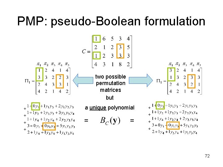
PMP: pseudo-Boolean formulation two possible permutation matrices but = = + + a unique polynomial 72

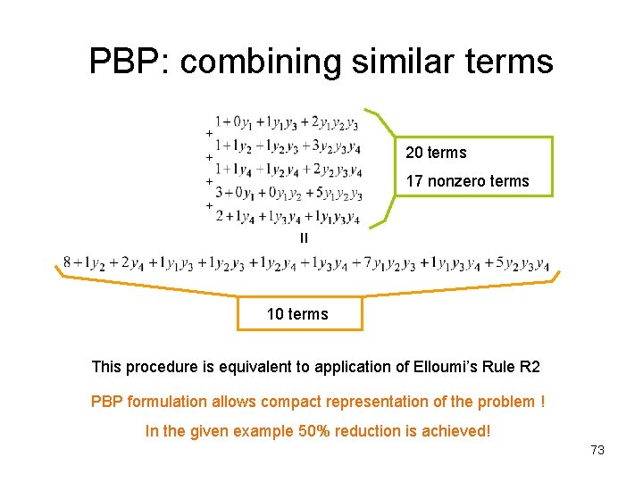
PBP: combining similar terms + + 20 terms = 17 nonzero terms 10 terms This procedure is equivalent to application of Elloumi’s Rule R 2 PBP formulation allows compact representation of the problem ! In the given example 50% reduction is achieved! 73

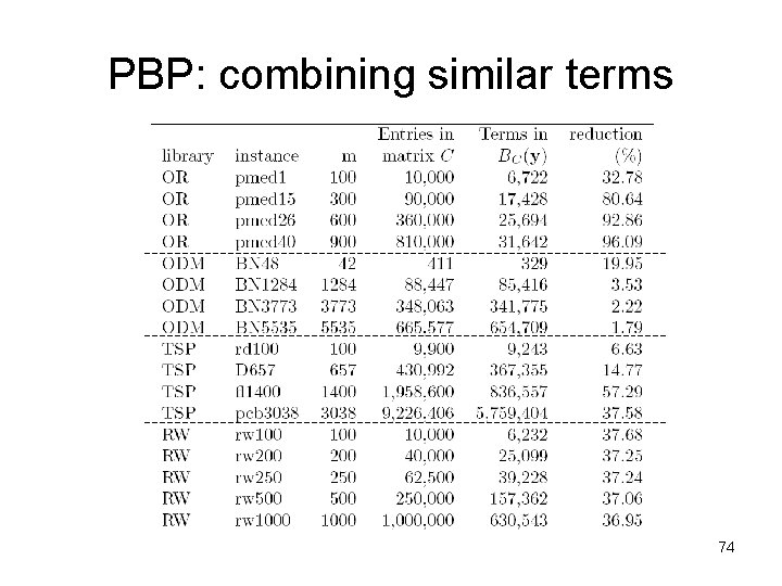
PBP: combining similar terms 74

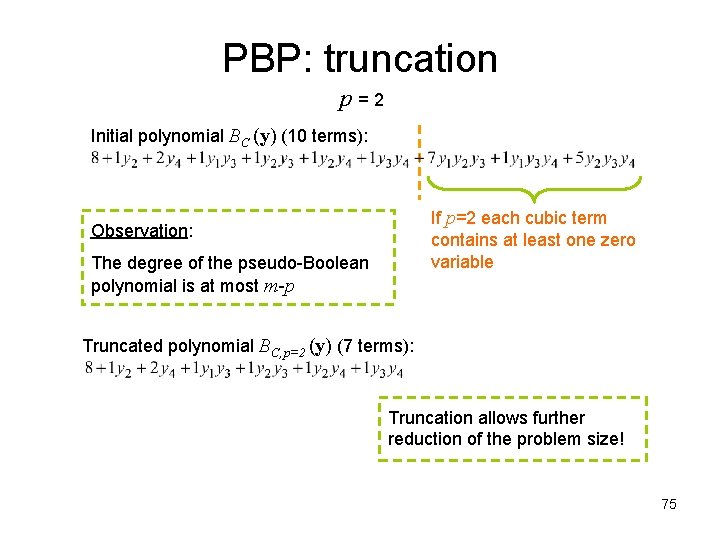
PBP: truncation p = 2 Initial polynomial BC (y) (10 terms): If p=2 each cubic term contains at least one zero variable Observation: The degree of the pseudo-Boolean polynomial is at most m-p Truncated polynomial BC, p=2 (y) (7 terms): Truncation allows further reduction of the problem size! 75

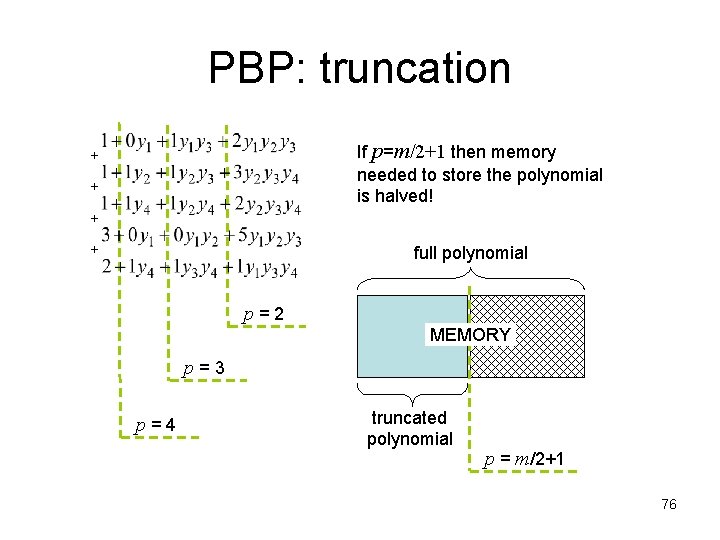
PBP: truncation + + If p=m/2+1 then memory needed to store the polynomial is halved! full polynomial p = 2 MEMORY p = 3 p = 4 truncated polynomial p = m/2+1 76

PMP: pseudo-Boolean formulation + + 77

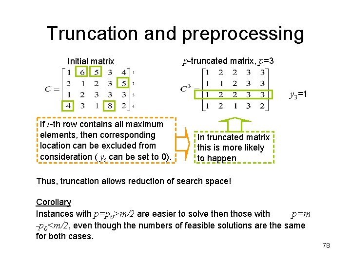
Truncation and preprocessing Initial matrix p-truncated matrix, p=3 y 3=1 If i-th row contains all maximum elements, then corresponding location can be excluded from consideration ( yi can be set to 0). In truncated matrix this is more likely to happen Thus, truncation allows reduction of search space! Corollary Instances with p=p 0>m/2 are easier to solve then those with p=m -p 0<m/2, even though the numbers of feasible solutions are the same for both cases. 78

Pseudo-Boolean formulation: outcomes • Compact but nonlinear problem • Equivalent to a nonlinear knapsack (NPhard) • Goal: obtain a model suitable for generalpurpose MILP solvers, e. g. : – – – CPLEX Xpress. MP MOSEK LPSOL CLP 79

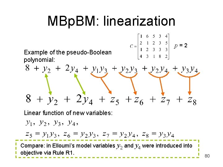
MBp. BM: linearization p = 2 Example of the pseudo-Boolean polynomial: Linear function of new variables: Compare: in Elloumi’s model variables y 2 and y 4 were introduced into objective via Rule R 1. 80

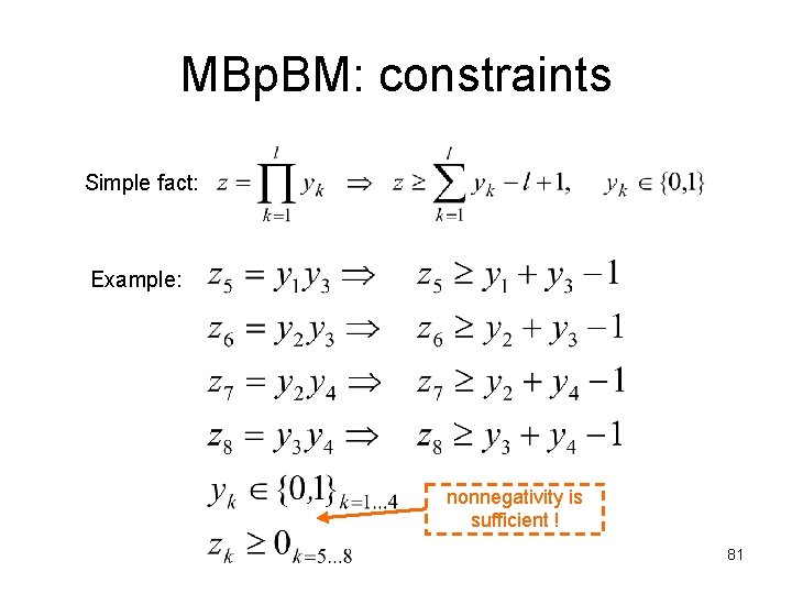
MBp. BM: constraints Simple fact: Example: nonnegativity is sufficient ! 81

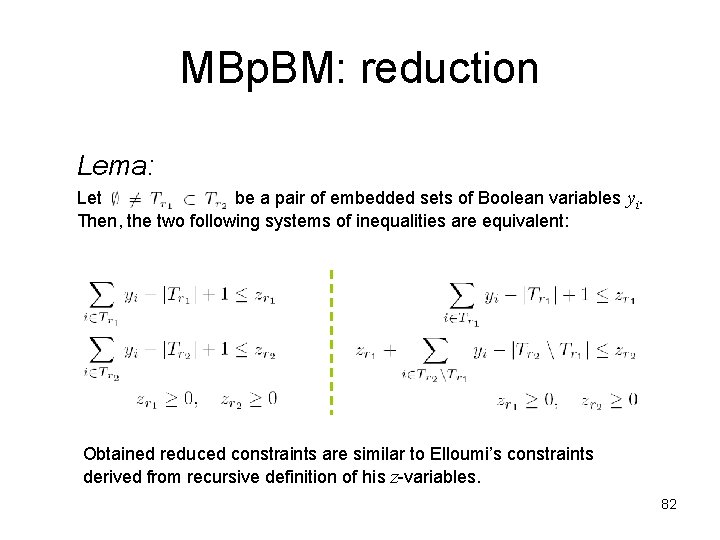
MBp. BM: reduction Lema: Let Ø be a pair of embedded sets of Boolean variables yi. Then, the two following systems of inequalities are equivalent: Obtained reduced constraints are similar to Elloumi’s constraints derived from recursive definition of his z-variables. 82

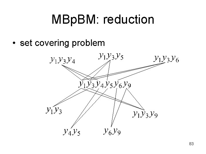
MBp. BM: reduction • set covering problem 83

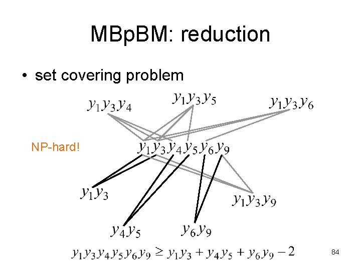
MBp. BM: reduction • set covering problem NP-hard! 84

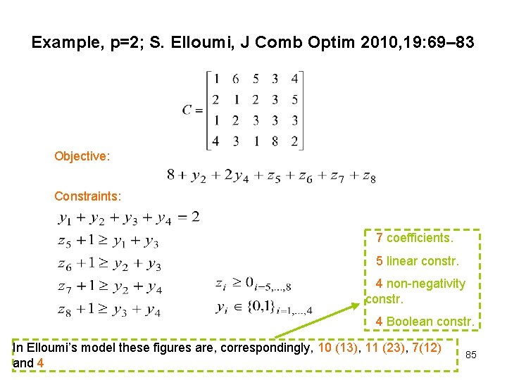
Example, p=2; S. Elloumi, J Comb Optim 2010, 19: 69– 83 Objective: Constraints: 7 coefficients. 5 linear constr. 4 non-negativity constr. 4 Boolean constr. In Elloumi’s model these figures are, correspondingly, 10 (13), 11 (23), 7(12) and 4 85

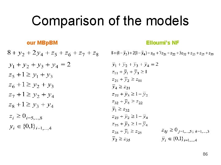
Comparison of the models our MBp. BM Elloumi’s NF 86

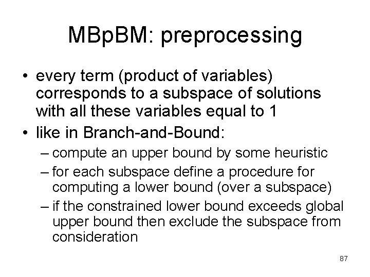
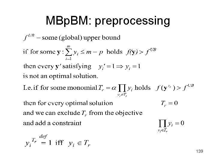
MBp. BM: preprocessing • every term (product of variables) corresponds to a subspace of solutions with all these variables equal to 1 • like in Branch-and-Bound: – compute an upper bound by some heuristic – for each subspace define a procedure for computing a lower bound (over a subspace) – if the constrained lower bound exceeds global upper bound then exclude the subspace from consideration 87

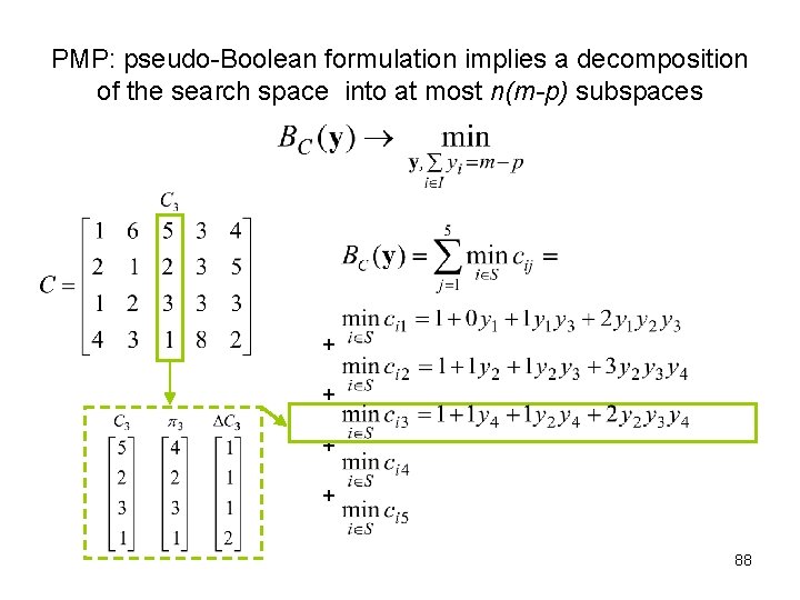
PMP: pseudo-Boolean formulation implies a decomposition of the search space into at most n(m-p) subspaces + + 88

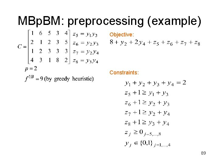
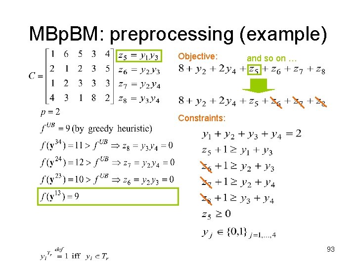
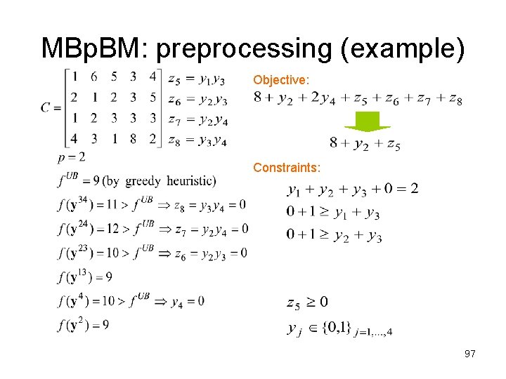
MBp. BM: preprocessing (example) Objective: Constraints: 89

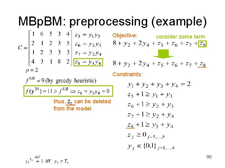
MBp. BM: preprocessing (example) Objective: consider some term Constraints: thus, z 8 can be deleted from the model 90

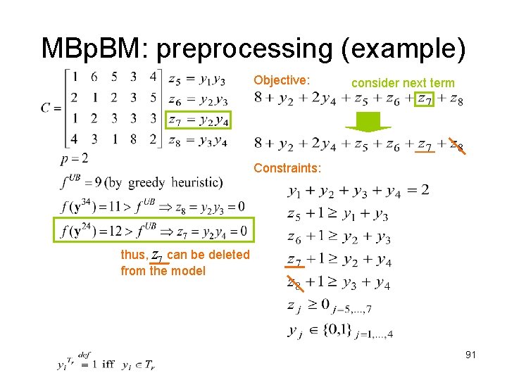
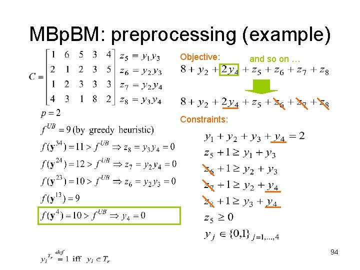
MBp. BM: preprocessing (example) Objective: consider next term Constraints: thus, z 7 can be deleted from the model 91

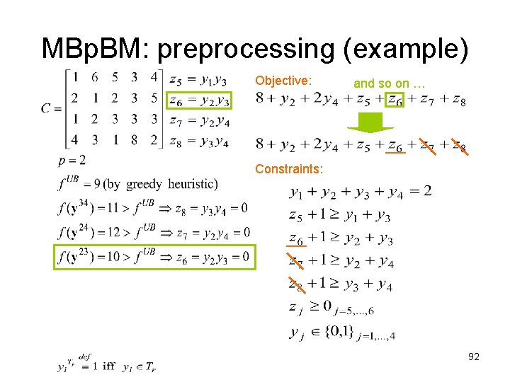
MBp. BM: preprocessing (example) Objective: and so on … Constraints: 92

MBp. BM: preprocessing (example) Objective: and so on … Constraints: 93

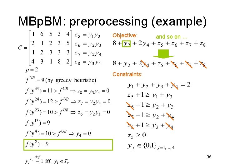
MBp. BM: preprocessing (example) Objective: and so on … Constraints: 94

MBp. BM: preprocessing (example) Objective: and so on … Constraints: 95

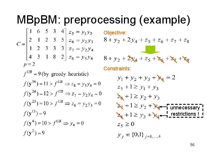
MBp. BM: preprocessing (example) Objective: Constraints: unnecessary restrictions ! 96

MBp. BM: preprocessing (example) Objective: Constraints: 97

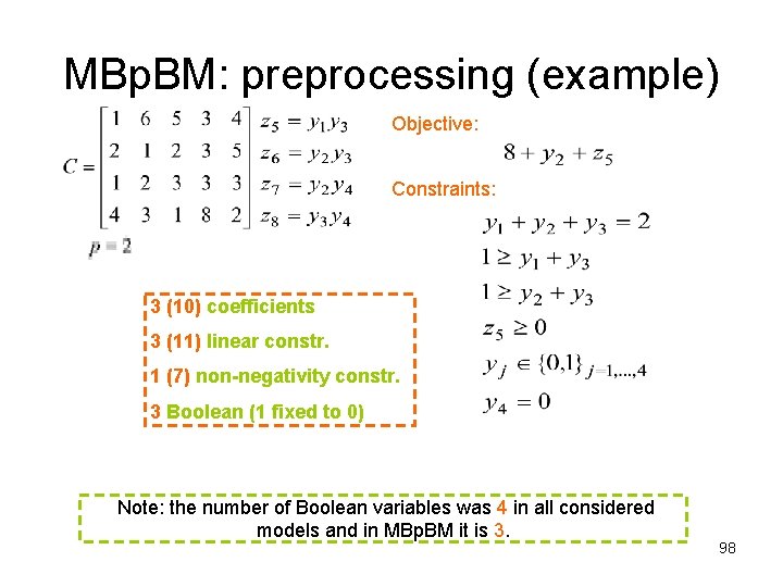
MBp. BM: preprocessing (example) Objective: Constraints: 3 (10) coefficients 3 (11) linear constr. 1 (7) non-negativity constr. 3 Boolean (1 fixed to 0) Note: the number of Boolean variables was 4 in all considered models and in MBp. BM it is 3. 98

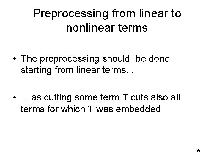
Preprocessing from linear to nonlinear terms • The preprocessing should be done starting from linear terms. . . • . . . as cutting some term T cuts also all terms for which T was embedded 99

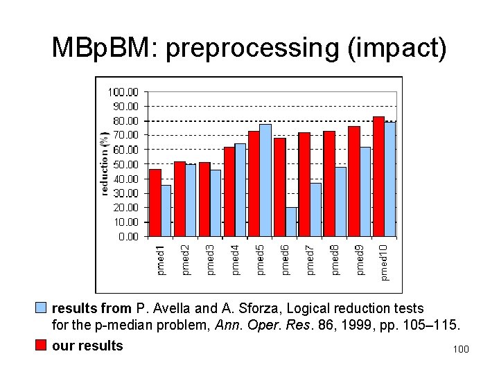
MBp. BM: preprocessing (impact) results from P. Avella and A. Sforza, Logical reduction tests for the p-median problem, Ann. Oper. Res. 86, 1999, pp. 105– 115. our results 100

Computational results OR-library instances [3] Avella P. , Sassano A. , Vasil’ev I. : Computational study of large-scale p-median problems. Math. Prog. , Ser. A, 109, 89 -114 (2007) [12] Church R. L. : BEAMR: An exact and approximate model for the p-median problem. Comp. & Oper. Res. , 35, 417 -426 (2008) [15] Elloumi S. : A tighter formulation of the p-median problem. J. Comb. Optim. , 19, 69– 83 (2010) 101

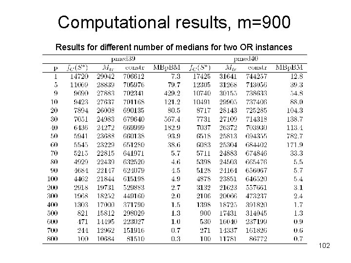
Computational results, m=900 Results for different number of medians for two OR instances 102

Computational results Results for different numbers of medians in BN 1284 [3] Avella P. , Sassano A. , Vasil’ev I. : Computational study of large-scale p-median problems. Math. Prog. , Ser. A, 109, 89 -114 (2007) 103

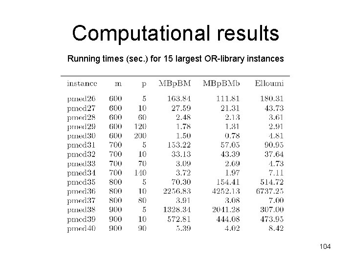
Computational results Running times (sec. ) for 15 largest OR-library instances 104

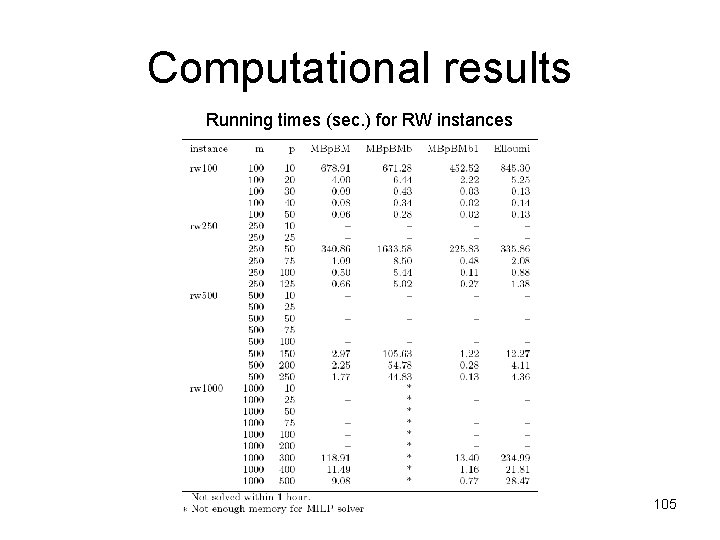
Computational results Running times (sec. ) for RW instances 105

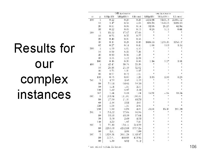
Results for our complex instances 106

Concluding remarks • a new Mixed Boolean Pseudo-Boolean linear programming Model (MBp. BM) for the p-median problem (PMP): Ø instance specific Ø optimal within the class of mixed Boolean LP models Ø allows solving previously unsolved instances with general purpose software 107

Future research directions • compact models for other location problems (e. g. SPLP or generalized PMP) • revised data-correcting approach • implementation and computational experiments with preprocessed MBp. BM based on lower and upper bounds 108

Next two lectures • How many instances do we really solve when solving a PMP instance • Why some data lead to more complex problems than other • Two applications in details 109

Literature • • • B. F. Al. Bdaiwi, B. Goldengorin, G. Sierksma. Equivalent instances of the simple plant location problem. Computers and Mathematics with Applications, 57 812— 820 (2009). B. F. Al. Bdaiwi, D. Ghosh, B. Goldengorin. Data Aggregation for p-Median Problems. Journal of Combinatorial Optimization 2010 (open access, in press) DOI: 10. 1007/s 10878 -009 -9251 -8. Avella, P. , Sforza, A. : Logical reduction tests for the p-median problem. Annals of Operations Research, 86, 105 -115 (1999). • Avella, P. , Sassano, A. , Vasil'ev, I. : Computational study of large-scale p -median problems. Mathematical Programming, Ser. A, 109, 89 -114 • • • (2007). Beresnev, V. L. On a Problem of Mathematical Standardization Theory, Upravliajemyje Sistemy, 11, 43– 54 (1973), (in Russian). Church, R. L. : BEAMR: An exact and approximate model for the p-median problem. Computers & Operations Research, 35, 417 -426 (2008). Cornuejols, G. , Nemhauser, G. , Wolsey, L. A. : A canonical representation of simple plant location problems and its applications. SIAM Journal on Matrix Analysis and Applications (SIMAX), 1(3), 261 -272 (1980). 110

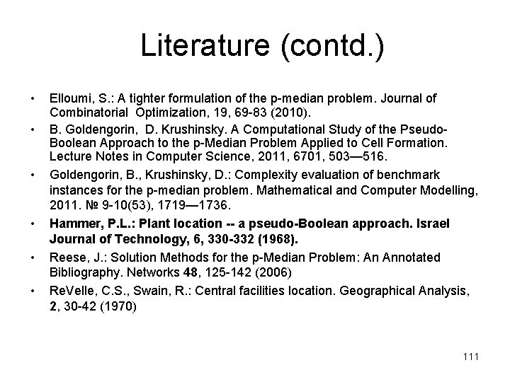
Literature (contd. ) • • • Elloumi, S. : A tighter formulation of the p-median problem. Journal of Combinatorial Optimization, 19, 69 -83 (2010). B. Goldengorin, D. Krushinsky. A Computational Study of the Pseudo. Boolean Approach to the p-Median Problem Applied to Cell Formation. Lecture Notes in Computer Science, 2011, 6701, 503— 516. Goldengorin, B. , Krushinsky, D. : Complexity evaluation of benchmark instances for the p-median problem. Mathematical and Computer Modelling, 2011. № 9 -10(53), 1719— 1736. Hammer, P. L. : Plant location -- a pseudo-Boolean approach. Israel Journal of Technology, 6, 330 -332 (1968). Reese, J. : Solution Methods for the p-Median Problem: An Annotated Bibliography. Networks 48, 125 -142 (2006) Re. Velle, C. S. , Swain, R. : Central facilities location. Geographical Analysis, 2, 30 -42 (1970) 111

Thank you! QUESTIONS? 112

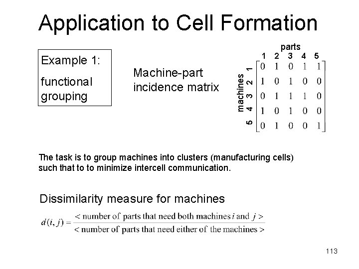
Application to Cell Formation 4 5 1 3 2 3 Machine-part incidence matrix 2 5 4 functional grouping 1 machines Example 1: parts The task is to group machines into clusters (manufacturing cells) such that to to minimize intercell communication. Dissimilarity measure for machines 113

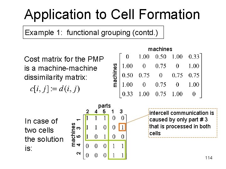
Application to Cell Formation Example 1: functional grouping (contd. ) Cost matrix for the PMP is a machine-machine dissimilarity matrix: 4 5 1 3 intercell communication is caused by only part # 3 that is processed in both cells 2 4 5 3 machines In case of two cells the solution is: 1 2 parts machines 114

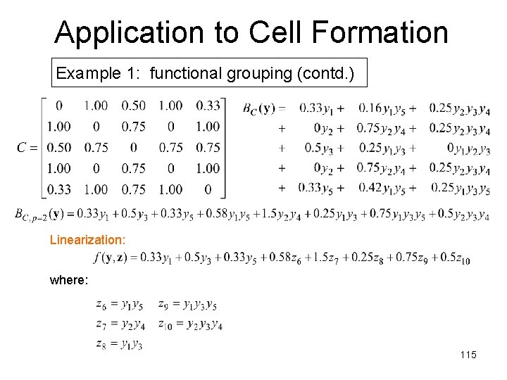
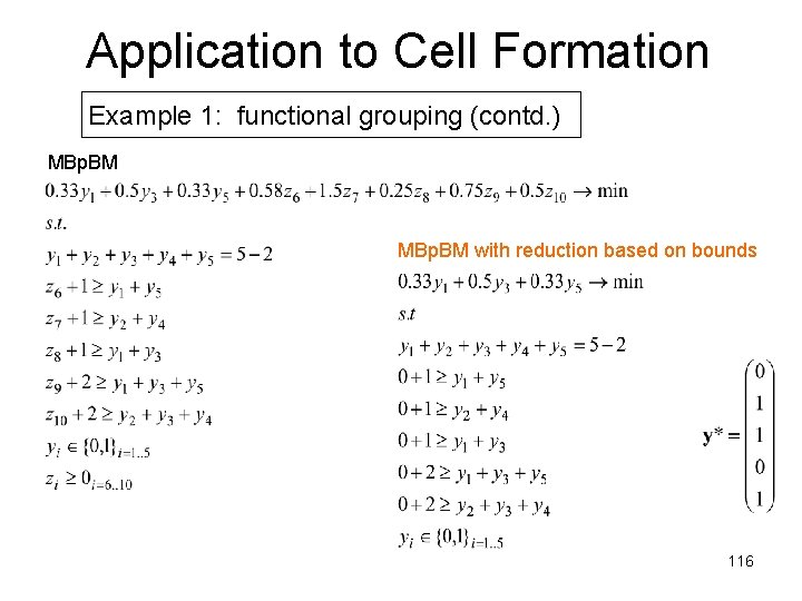
Application to Cell Formation Example 1: functional grouping (contd. ) Linearization: where: 115

Application to Cell Formation Example 1: functional grouping (contd. ) MBp. BM with reduction based on bounds 116

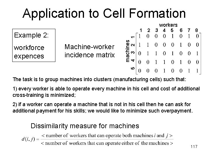
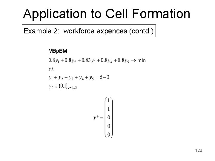
Application to Cell Formation 1 4 5 6 7 8 2 3 4 5 Machine-worker incidence matrix machines workforce expences 3 1 Example 2: 2 workers The task is to group machines into clusters (manufacturing cells) such that: 1) every worker is able to operate every machine in his cell and cost of additional cross-training is minimized; 2) if a worker can operate a machine that is not in his cell then he can ask for additional payment for his skills; we would like to minimize such overpayment. Dissimilarity measure for machines 117

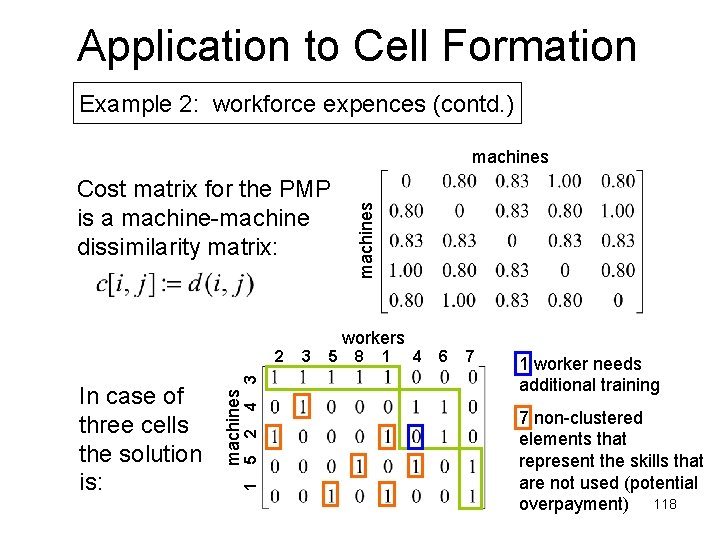
Application to Cell Formation Example 2: workforce expences (contd. ) Cost matrix for the PMP is a machine-machine dissimilarity matrix: 1 5 2 4 machines In case of three cells the solution is: 3 2 3 5 machines workers 8 1 4 6 7 1 worker needs additional training 7 non-clustered elements that represent the skills that are not used (potential overpayment) 118

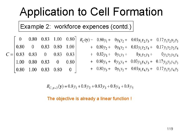
Application to Cell Formation Example 2: workforce expences (contd. ) The objective is already a linear function ! 119

Application to Cell Formation Example 2: workforce expences (contd. ) MBp. BM 120

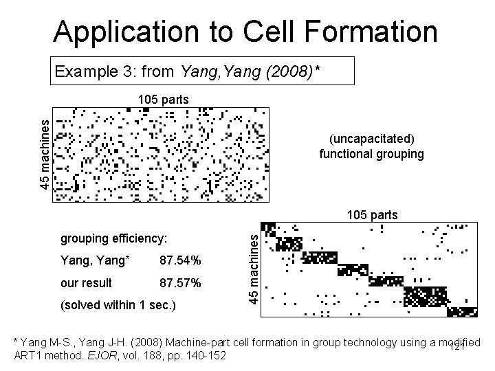
Application to Cell Formation Example 3: from Yang, Yang (2008)* 45 machines 105 parts (uncapacitated) functional grouping efficiency: Yang, Yang* 87. 54% our result 87. 57% (solved within 1 sec. ) 45 machines 105 parts * Yang M-S. , Yang J-H. (2008) Machine-part cell formation in group technology using a modified 121 ART 1 method. EJOR, vol. 188, pp. 140 -152

Thank you! • Questions? 122

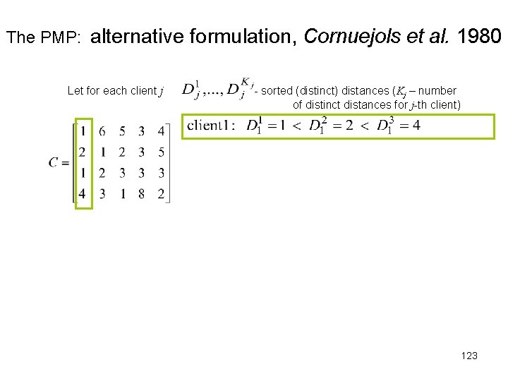
The PMP: alternative formulation, Cornuejols et al. 1980 Let for each client j - sorted (distinct) distances (Kj – number of distinct distances for j-th client) 123

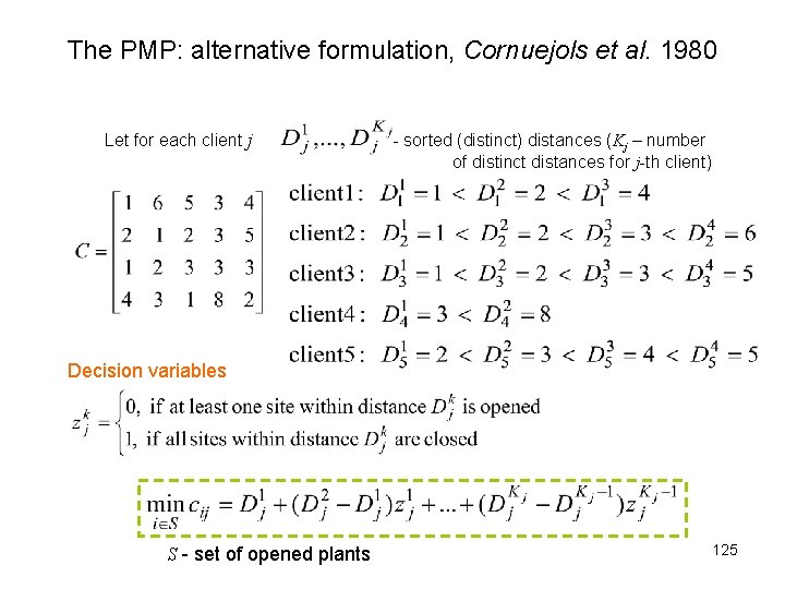
The PMP: alternative formulation, Cornuejols et al. 1980 Let for each client j - sorted (distinct) distances (Kj – number of distinct distances for j-th client) 124

The PMP: alternative formulation, Cornuejols et al. 1980 Let for each client j - sorted (distinct) distances (Kj – number of distinct distances for j-th client) Decision variables S - set of opened plants 125

The PMP: alternative formulation, Cornuejols et al. 1980 s. t. - p opened facilities - either at least one facility is open within or - for every client it is an opened facility in some neighbourhood - iff all the sites within are closed for each client i - sorted distances 126

The PMP: alternative formulation, Cornuejols et al. 1980 Example (Elloumi, 2009) Objective: + + only distinct (in a column) distances are meaningful 13 coefficients 127

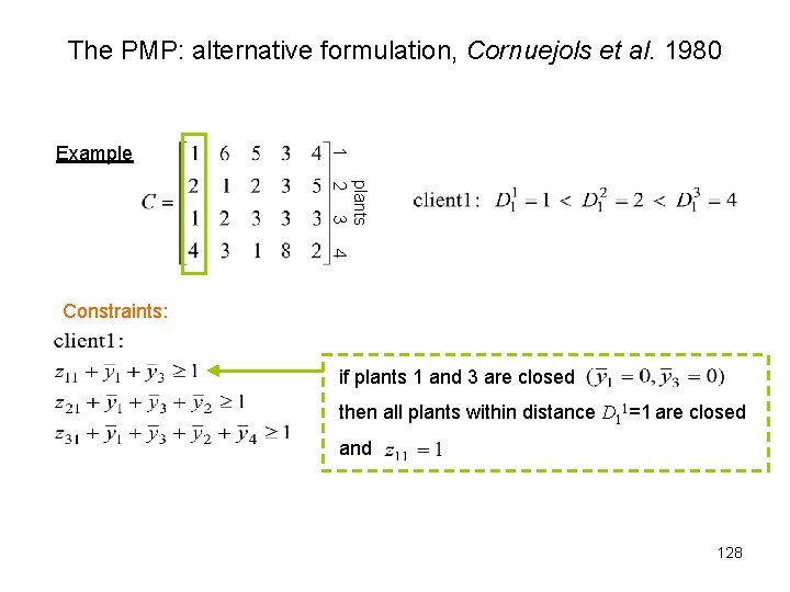
The PMP: alternative formulation, Cornuejols et al. 1980 plants 1 2 3 4 Example Constraints: if plants 1 and 3 are closed then all plants within distance D 11=1 are closed and 128

The PMP: alternative formulation, Cornuejols et al. 1980 Example (Elloumi, 2009) Objective: + + only distinct (in a column) distances are meaningful 13 coefficients 129

The PMP: alternative formulation, Cornuejols et al. 1980 Example Objective: Constraints: 13 coefficients, 23 linear constr. , 12 non-negativity constr. , 4 Boolean 130

The PMP: a tighter formulation, Elloumi 2009 A possible definition of variables : Or recursively: Thus: 131

The PMP: a tighter formulation, Elloumi 2009 s. t. Cornuejols et al. 1980 for each client j - sorted distances 132

The PMP: a tighter formulation, Elloumi 2009 Informally: if for client j some neighbourhood k contains only one facility i then there is a simple relation between corresponding variables 133

The PMP: a tighter formulation, Elloumi 2009 Informally: if two clients have equal neighbourhoods then the corresponding z-variables are equivalent and in the objective function terms containing them can be added. 134

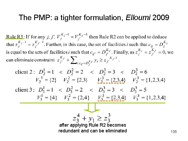
The PMP: a tighter formulation, Elloumi 2009 after applying Rule R 2 becomes redundant and can be eliminated 135

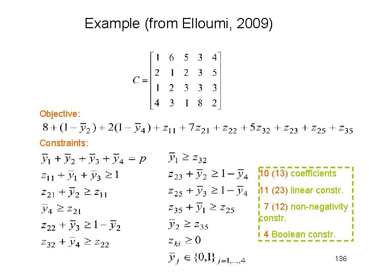
Example (from Elloumi, 2009) Objective: Constraints: 10 (13) coefficients 11 (23) linear constr. 7 (12) non-negativity constr. 4 Boolean constr. 136

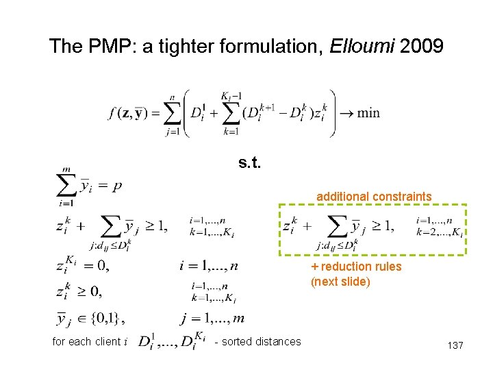
The PMP: a tighter formulation, Elloumi 2009 s. t. additional constraints + reduction rules (next slide) for each client i - sorted distances 137

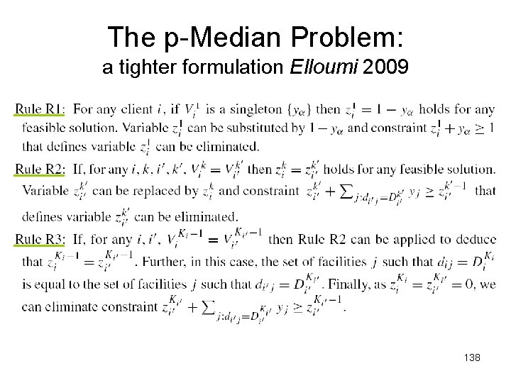
The p-Median Problem: a tighter formulation Elloumi 2009 138

MBp. BM: preprocessing 139

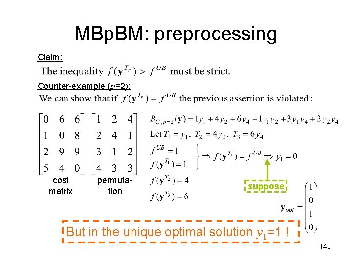
MBp. BM: preprocessing Claim: Counter-example (p=2): cost matrix permutation suppose But in the unique optimal solution y 1=1 ! 140