Mixed Cost Analysis Fixed And Variable Costs Cost

Mixed Cost Analysis

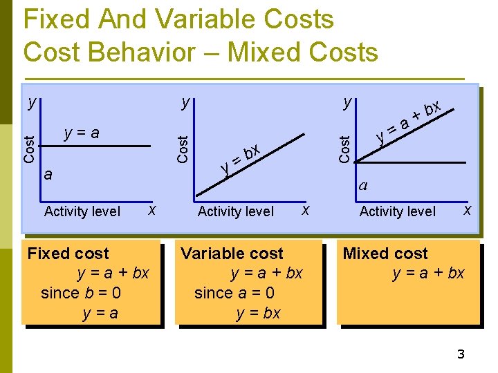
Fixed And Variable Costs Cost Behavior – Mixed Costs y Cost y=a a Activity level x Fixed cost y = a + bx since b = 0 y=a y y x b = Activity level a = y Cost y x b + a x Variable cost y = a + bx since a = 0 y = bx Activity level x Mixed cost y = a + bx 3

Methods of Analysis p Scatter diagram p High-low method p Linear regression analysis 4

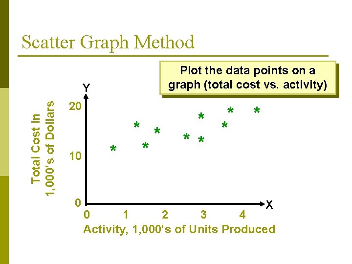
Scatter Graph Method Plot the data points on a graph (total cost vs. activity) Total Cost in 1, 000’s of Dollars Y 20 10 0 * * ** X 0 1 2 3 4 Activity, 1, 000’s of Units Produced

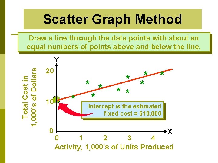
Scatter Graph Method Draw a line through the data points with about an equal numbers of points above and below the line. Total Cost in 1, 000’s of Dollars Y 20 10 * ** * * Intercept is the estimated fixed cost = $10, 000 0 X 0 1 2 3 4 Activity, 1, 000’s of Units Produced

Advantages and Disadvantages p One of the principal advantages of this method is that it lets us “see” the data. p Shows the correlation between costs and volume of activity p Apply with caution because it does not provide and objective test that the line drawn is the most accurate.

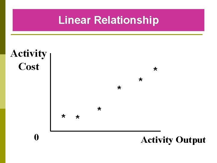
Linear Relationship Activity Cost * * * 0 * * * Activity Output

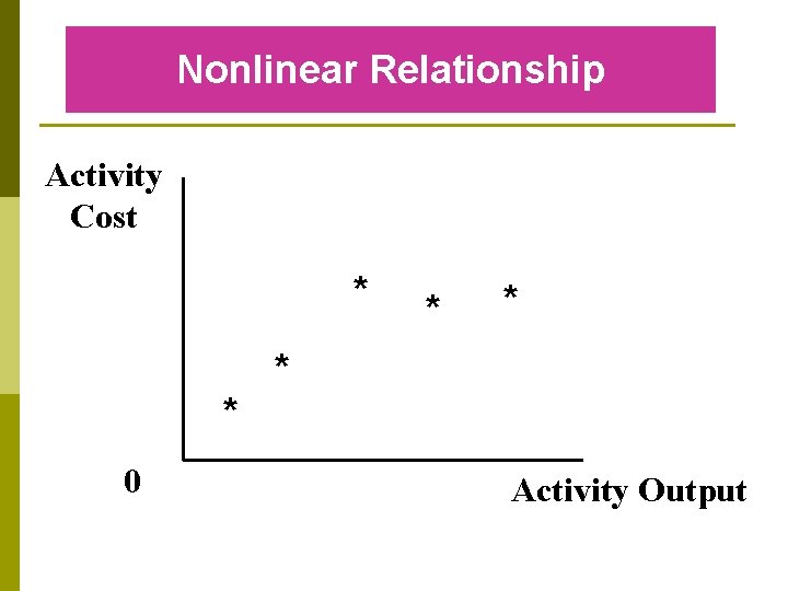
Nonlinear Relationship Activity Cost * * * 0 Activity Output

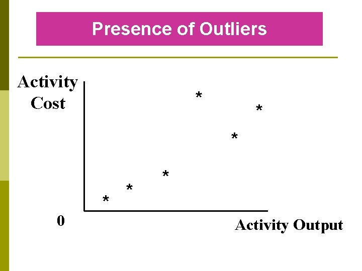
Presence of Outliers Activity Cost * * * 0 * * * Activity Output

Scatter Graph Example The sales manager for Hinds Wholesale Supply Company needs to estimate the expected delivery vehicle operating cost (maintenance) for 2014.

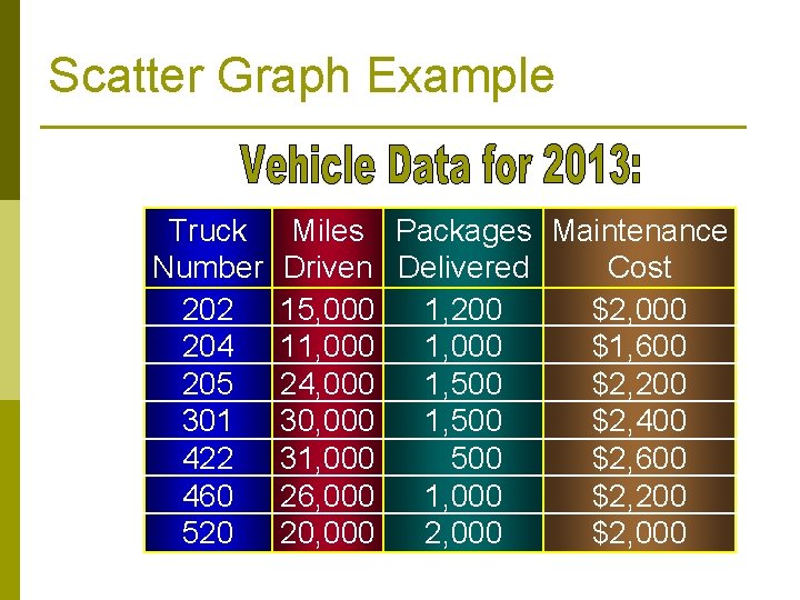
Scatter Graph Example Truck Number 202 204 205 301 422 460 520 Miles Packages Maintenance Driven Delivered Cost 15, 000 1, 200 $2, 000 11, 000 $1, 600 24, 000 1, 500 $2, 200 30, 000 1, 500 $2, 400 31, 000 500 $2, 600 26, 000 1, 000 $2, 200 20, 000 2, 000 $2, 000

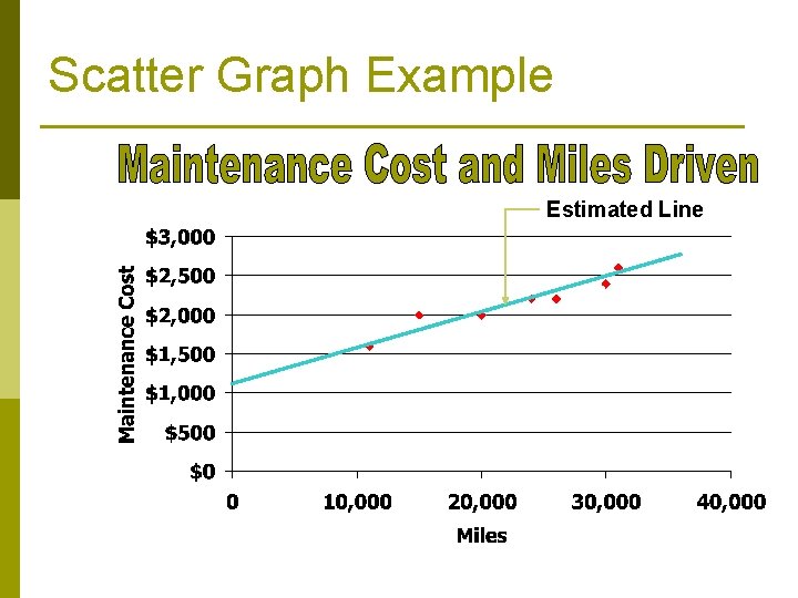
Scatter Graph Example Estimated Line

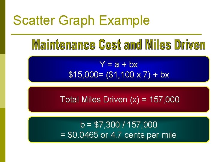
Scatter Graph Example Y = a + bx $15, 000= ($1, 100 x 7) + bx Total Miles Driven (x) = 157, 000 b = $7, 300 / 157, 000 = $0. 0465 or 4. 7 cents per mile

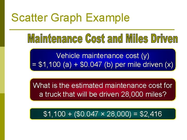
Scatter Graph Example Vehicle maintenance cost (y) = $1, 100 (a) + $0. 047 (b) per mile driven (x) What is the estimated maintenance cost for a truck that will be driven 28, 000 miles? $1, 100 + ($0. 047 × 28, 000) = $2, 416

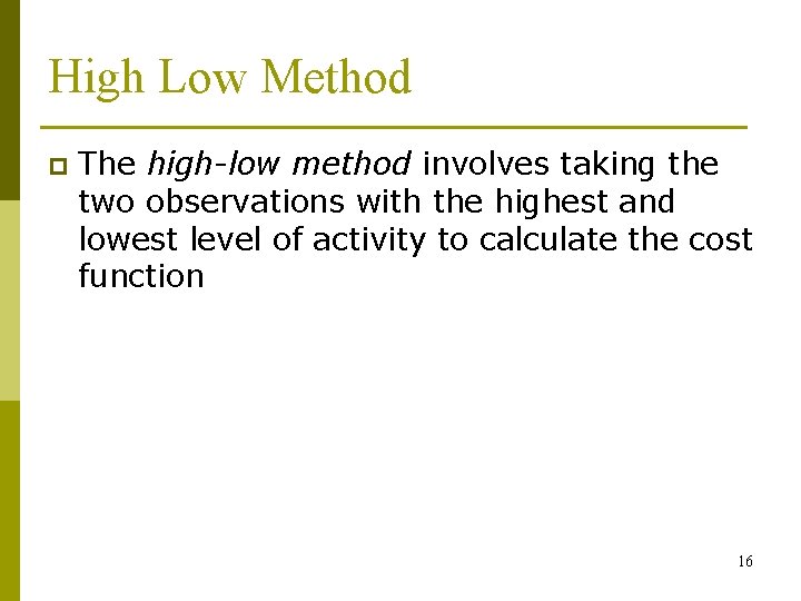
High Low Method p The high-low method involves taking the two observations with the highest and lowest level of activity to calculate the cost function 16

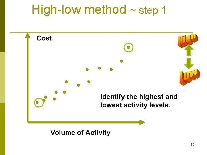
High-low method ~ step 1 Cost Identify the highest and lowest activity levels. Volume of Activity 17

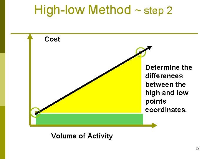
High-low Method ~ step 2 Cost Determine the differences between the high and low points coordinates. Volume of Activity 18

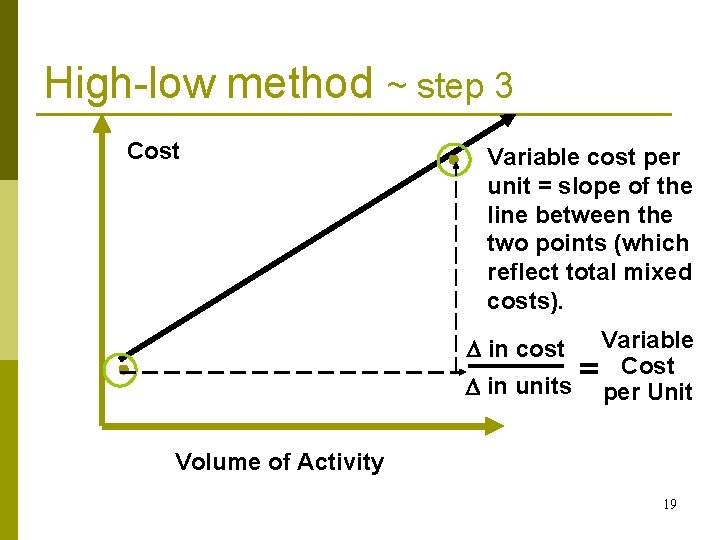
High-low method ~ step 3 Cost Variable cost per unit = slope of the line between the two points (which reflect total mixed costs). Variable Cost = in units per Unit in cost Volume of Activity 19

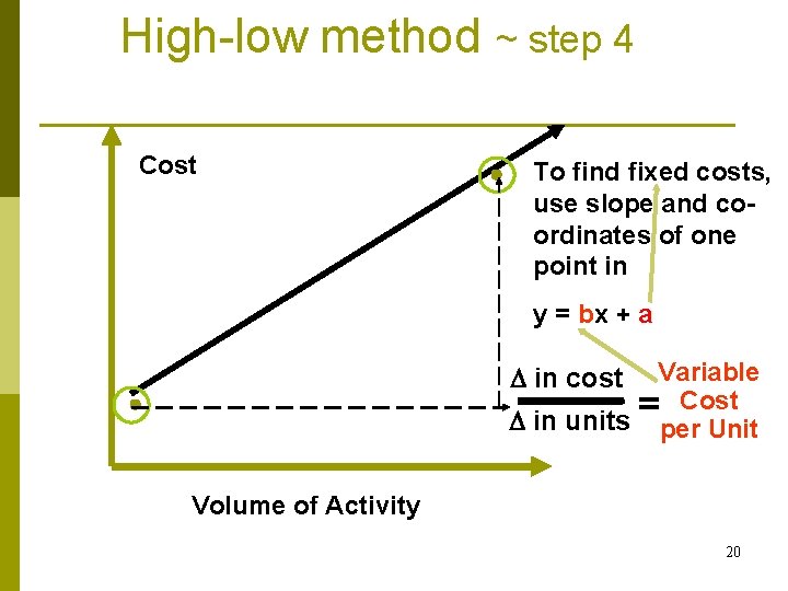
High-low method ~ step 4 Cost To find fixed costs, use slope and coordinates of one point in y = bx + a Variable Cost = in units per Unit in cost Volume of Activity 20

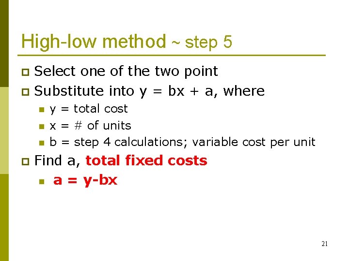
High-low method ~ step 5 Select one of the two point p Substitute into y = bx + a, where p n n n p y = total cost x = # of units b = step 4 calculations; variable cost per unit Find a, total fixed costs n a = y-bx 21

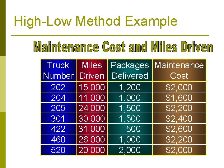
High-Low Method Example Truck Number 202 204 205 301 422 460 520 Miles Packages Maintenance Driven Delivered Cost 15, 000 1, 200 $2, 000 11, 000 $1, 600 24, 000 1, 500 $2, 200 30, 000 1, 500 $2, 400 31, 000 500 $2, 600 26, 000 1, 000 $2, 200 20, 000 2, 000 $2, 000

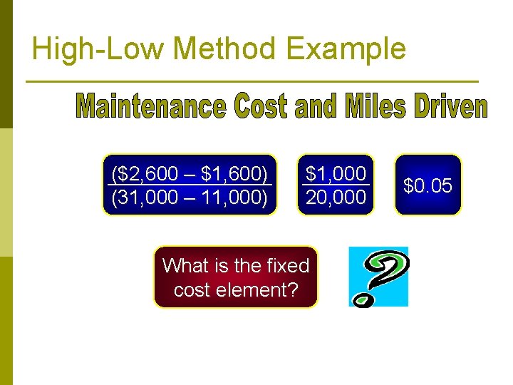
High-Low Method Example ($2, 600 – $1, 600) $1, 000 = = $0. 05 (31, 000 – 11, 000) 20, 000 What is the fixed cost element?

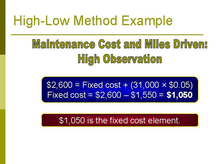
High-Low Method Example $2, 600 = Fixed cost + (31, 000 × $0. 05) Fixed cost = $2, 600 – $1, 550 = $1, 050 is the fixed cost element.

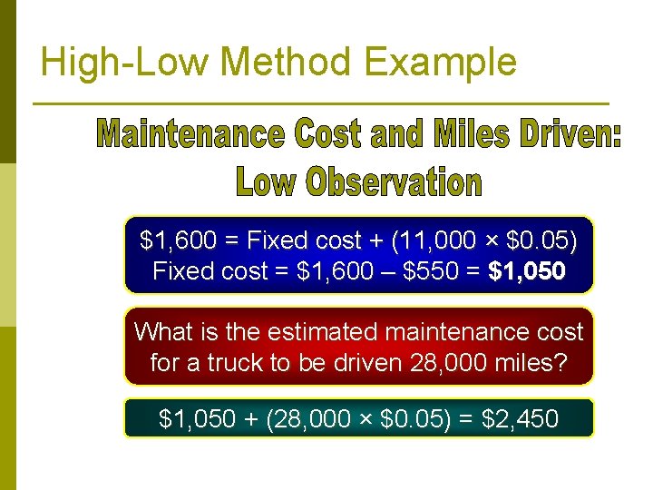
High-Low Method Example $1, 600 = Fixed cost + (11, 000 × $0. 05) Fixed cost = $1, 600 – $550 = $1, 050 What is the estimated maintenance cost for a truck to be driven 28, 000 miles? $1, 050 + (28, 000 × $0. 05) = $2, 450

Strengths of High-Low Method p Simple p Easy to use to understand p Analysis based of easily accessible data (expenses and activity levels)

Weaknesses of High-Low p Rather unreliable, only two data points are used in the analysis. p Can be problematic if either (or both) high or low are extreme (i. e. , Outliers). p Number of steps, where each additional step increases the potential for errors.

End of Mixed Cost Analysis