Minimum Spanning Trees Definition of MST Generic MST

Minimum Spanning Trees Definition of MST Generic MST algorithm Kruskal's algorithm Prim's algorithm Binary Search Trees 1

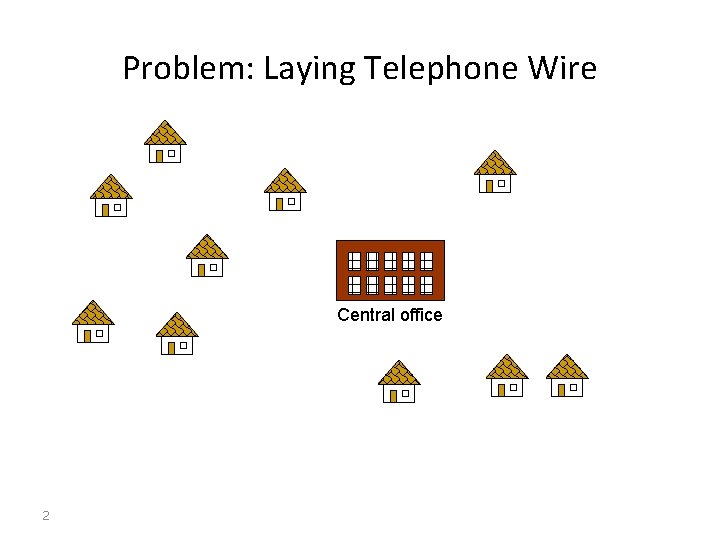
Problem: Laying Telephone Wire Central office 2

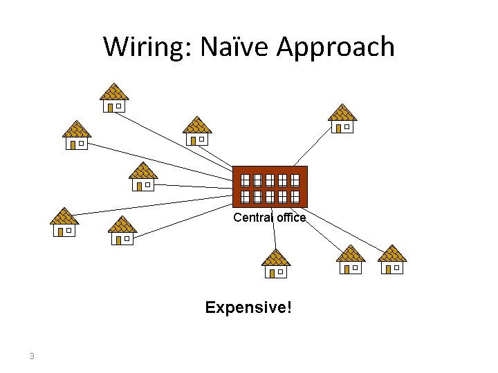
Wiring: Naïve Approach Central office Expensive! 3

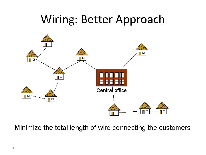
Wiring: Better Approach Central office Minimize the total length of wire connecting the customers 4

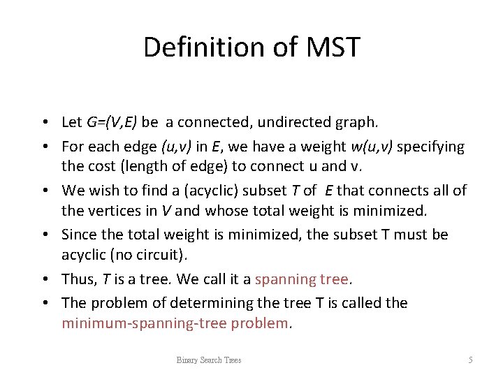
Definition of MST • Let G=(V, E) be a connected, undirected graph. • For each edge (u, v) in E, we have a weight w(u, v) specifying the cost (length of edge) to connect u and v. • We wish to find a (acyclic) subset T of E that connects all of the vertices in V and whose total weight is minimized. • Since the total weight is minimized, the subset T must be acyclic (no circuit). • Thus, T is a tree. We call it a spanning tree. • The problem of determining the tree T is called the minimum-spanning-tree problem. Binary Search Trees 5

Application of MST: an example • In the design of electronic circuitry, it is often necessary to make a set of pins electrically equivalent by wiring them together. • To interconnect n pins, we can use n-1 wires, each connecting two pins. • We want to minimize the total length of the wires. • Minimum Spanning Trees can be used to model this problem. Binary Search Trees 6

Electronic Circuits: Binary Search Trees 7

Electronic Circuits: Binary Search Trees 8

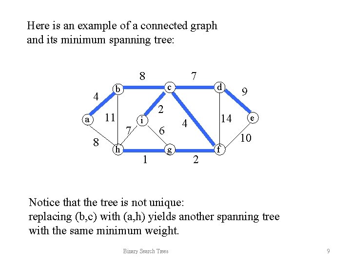
Here is an example of a connected graph and its minimum spanning tree: 8 4 8 c b 11 a h 7 i 1 7 d 2 14 4 6 g 2 f 9 e 10 Notice that the tree is not unique: replacing (b, c) with (a, h) yields another spanning tree with the same minimum weight. Binary Search Trees 9

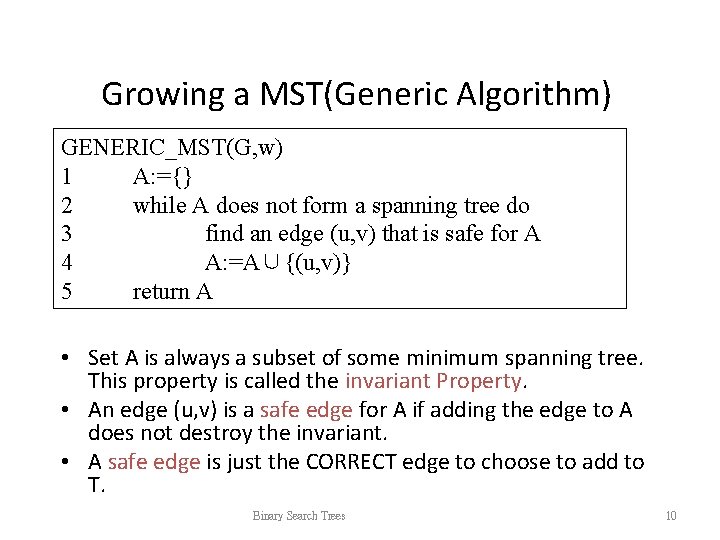
Growing a MST(Generic Algorithm) GENERIC_MST(G, w) 1 A: ={} 2 while A does not form a spanning tree do 3 find an edge (u, v) that is safe for A 4 A: =A∪{(u, v)} 5 return A • Set A is always a subset of some minimum spanning tree. This property is called the invariant Property. • An edge (u, v) is a safe edge for A if adding the edge to A does not destroy the invariant. • A safe edge is just the CORRECT edge to choose to add to T. Binary Search Trees 10

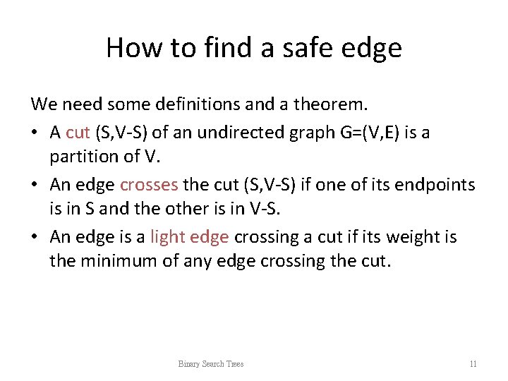
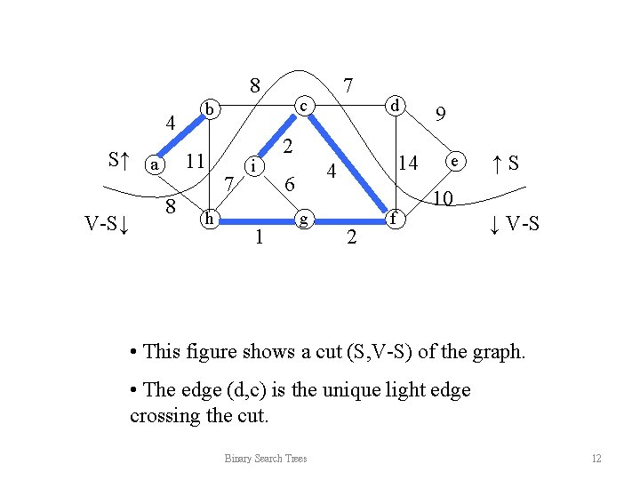
How to find a safe edge We need some definitions and a theorem. • A cut (S, V-S) of an undirected graph G=(V, E) is a partition of V. • An edge crosses the cut (S, V-S) if one of its endpoints is in S and the other is in V-S. • An edge is a light edge crossing a cut if its weight is the minimum of any edge crossing the cut. Binary Search Trees 11

8 4 S↑ a V-S↓ 8 c b 11 h 7 i 1 7 d 2 14 4 6 g 2 f 9 e ↑S 10 ↓ V-S • This figure shows a cut (S, V-S) of the graph. • The edge (d, c) is the unique light edge crossing the cut. Binary Search Trees 12

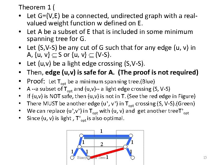
Theorem 1 ( • Let G=(V, E) be a connected, undirected graph with a realvalued weight function w defined on E. • Let A be a subset of E that is included in some minimum spanning tree for G. • Let (S, V-S) be any cut of G such that for any edge (u, v) in A, {u, v} S or {u, v} (V-S). • Let (u, v) be a light edge crossing (S, V-S). • Then, edge (u, v) is safe for A. (The proof is not required) • Proof: Let Topt be a minimum spanning tree. (Blue) • • • A --a subset of Topt and (u, v)-- a light edge crossing (S, V-S) If (u, v) is NOT safe, then (u, v) is not in T. (See the red edge in Figure) There MUST be another edge (u’, v’) in Topt crossing (S, V-S). (Green) We can replace (u’, v’) in Topt with (u, v) and get another tree. T’opt Since (u, v) is light , T’opt is also optimal. 1 1 1 2 1 Binary Search Trees 1 13

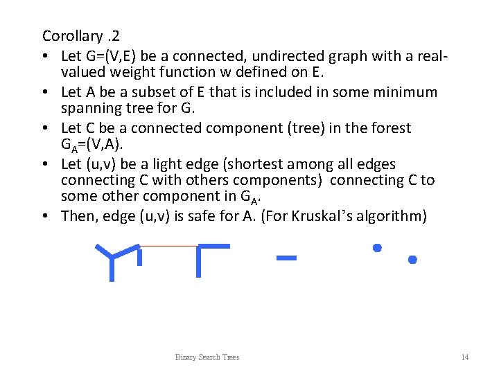
Corollary. 2 • Let G=(V, E) be a connected, undirected graph with a realvalued weight function w defined on E. • Let A be a subset of E that is included in some minimum spanning tree for G. • Let C be a connected component (tree) in the forest GA=(V, A). • Let (u, v) be a light edge (shortest among all edges connecting C with others components) connecting C to some other component in GA. • Then, edge (u, v) is safe for A. (For Kruskal’s algorithm) Binary Search Trees 14

Prim's algorithm(basic part) MST_PRIM(G, w, r) 1. A={} 2. S: ={r} (r is an arbitrary node in V) 3. Q=V-{r}; 4. while Q is not empty do { 5 take an edge (u, v) such that (1) u S and v Q (v S ) and (u, v) is the shortest edge satisfying (1) 6 add (u, v) to A, add v to S and delete v from Q } Binary Search Trees 15

Prim's algorithm MST_PRIM(G, w, r) 1 for each u in Q do 2 key[u]: =∞ 3 parent[u]: =NIL 4 key[r]: =0; parent[r]=NIL; 5 Q V[Q] 6 while Q!={} do 7 u: =EXTRACT_MIN(Q); if parent[u] Nil print (u, parent[u]) 8 for each v in Adj[u] do 9 if v in Q and w(u, v)<key[v] 10 then parent[v]: =u 11 key[v]: =w(u, v) Binary Search Trees 16

• Grow the minimum spanning tree from the root vertex r. • Q is a priority queue, holding all vertices that are not in the tree now. • key[v] is the minimum weight of any edge connecting v to a vertex in the tree. • parent[v] names the parent of v in the tree. • When the algorithm terminates, Q is empty; the minimum spanning tree A for G is thus A={(v, parent[v]): v∈V-{r}}. • Running time: O(||E||lg |V|). • When |E|=O(|V|), the algorithm is very fast. Binary Search Trees 17

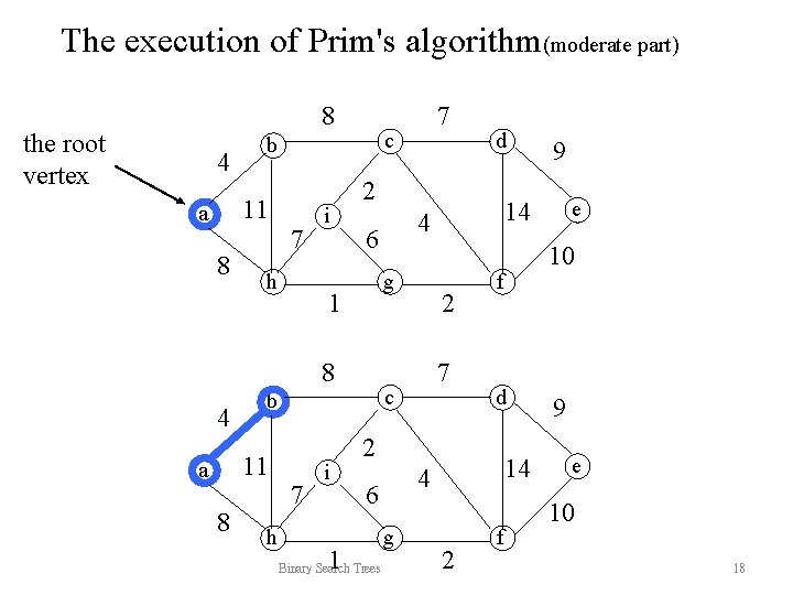
The execution of Prim's algorithm(moderate part) 8 the root vertex 4 8 c b 11 a 7 h i g 1 8 h 7 i 1 2 7 c d Binary Search Trees 14 4 g e 10 f 2 6 9 14 4 6 b 11 a d 2 8 4 7 2 f 9 e 10 18

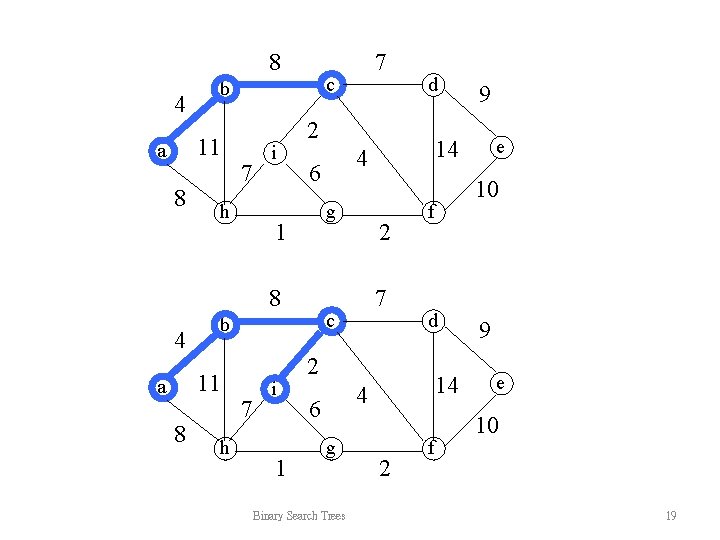
8 4 8 c b 11 a 7 h i g 1 8 h 7 i 1 2 7 c d 14 4 g Binary Search Trees e 10 f 2 6 9 14 4 6 b 11 a d 2 8 4 7 2 f 9 e 10 19

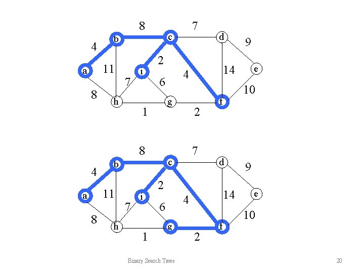
8 4 8 c b 11 a 7 h i g 1 8 h 7 i 1 2 7 c d 14 4 g Binary Search Trees e 10 f 2 6 9 14 4 6 b 11 a d 2 8 4 7 2 f 9 e 10 20

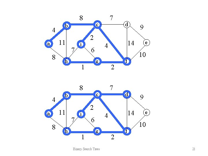
8 4 8 c b 11 a 7 h i g 1 8 h 7 i 1 2 7 c d 14 4 g Binary Search Trees e 10 f 2 6 9 14 4 6 b 11 a d 2 8 4 7 2 f 9 e 10 21

Adaptable Heap: • An adaptable heap is a heap that allows to change the key value of an entry in heap. – How to find the entry? – After changing the key value, how to make sure that the heap order holds. • We use array representation to store a complete binary tree. Binary Search Trees 22

Adaptable Heap: • Entry: (key, id, value), where key is a real number (double), value is a string (String) and id is an integer (int) indicating the entry. • Here id uniquely determine the entry. The value of id is from 1 to n if there are n entries in the priority queue. • For MST application, id is the name of a vertex in a graph. Value is the name of the other vertex of the edge that we will added into A. Binary Search Trees 23

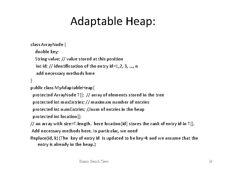
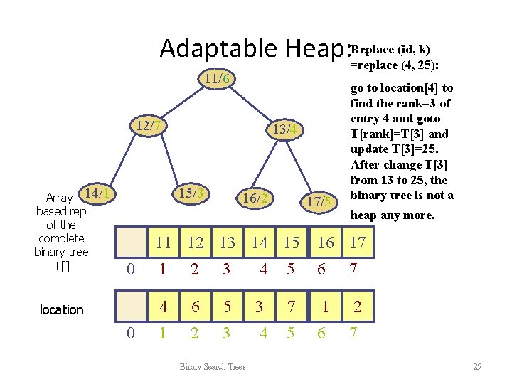
Adaptable Heap: class Array. Node { double key; String value; // value stored at this position int id; // identificsation of the entry id=1, 2, 3, …, n add necessary methods here } public class My. Adaptable. Heap{ protected Array. Node T[]; // array of elements stored in the tree protected int max. Entries; // maximum number of entries protected int num. Entries; //num of entries in the heap protected int location[]; // an array with size=T. length. here location[id] stores the rank of entry id in T[]. Add necessary methods here. In particular, we need Replace(id, k) (The key of entry id is updated to be key=k and we assume that the entry is already in the heap. ) Binary Search Trees 24

(id, k) Adaptable Heap: Replace =replace (4, 25): 11/6 12/7 Array- 14/1 based rep of the complete binary tree T[] 13/4 15/3 0 location 0 16/2 17/5 go to location[4] to find the rank=3 of entry 4 and goto T[rank]=T[3] and update T[3]=25. After change T[3] from 13 to 25, the binary tree is not a heap any more. 11 12 13 14 15 16 17 1 2 3 4 5 6 7 4 6 5 3 7 1 2 3 4 5 6 7 Binary Search Trees 25

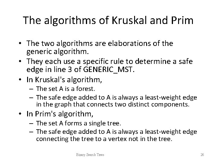
The algorithms of Kruskal and Prim • The two algorithms are elaborations of the generic algorithm. • They each use a specific rule to determine a safe edge in line 3 of GENERIC_MST. • In Kruskal's algorithm, – The set A is a forest. – The safe edge added to A is always a least-weight edge in the graph that connects two distinct components. • In Prim's algorithm, – The set A forms a single tree. – The safe edge added to A is always a least-weight edge connecting the tree to a vertex not in the tree. Binary Search Trees 26

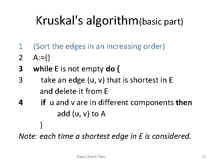
Kruskal's algorithm(basic part) 1 2 3 3 (Sort the edges in an increasing order) A: ={} while E is not empty do { take an edge (u, v) that is shortest in E and delete it from E 4 if u and v are in different components then add (u, v) to A } Note: each time a shortest edge in E is considered. Binary Search Trees 27

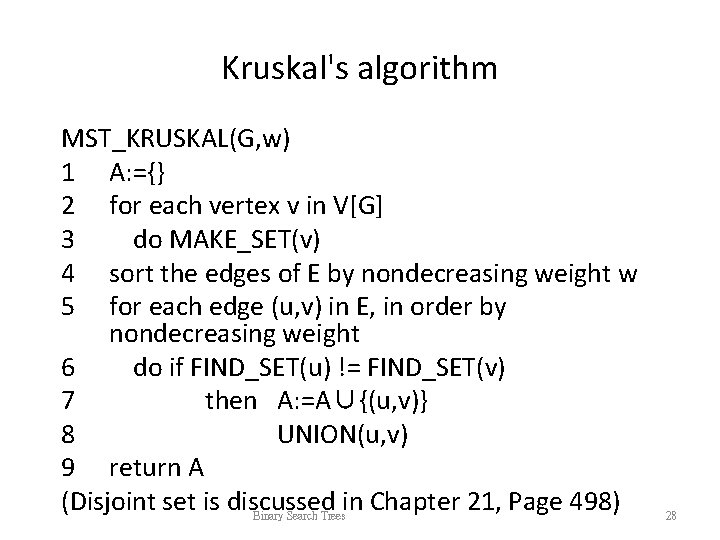
Kruskal's algorithm MST_KRUSKAL(G, w) 1 A: ={} 2 for each vertex v in V[G] 3 do MAKE_SET(v) 4 sort the edges of E by nondecreasing weight w 5 for each edge (u, v) in E, in order by nondecreasing weight 6 do if FIND_SET(u) != FIND_SET(v) 7 then A: =A∪{(u, v)} 8 UNION(u, v) 9 return A (Disjoint set is discussed in Chapter 21, Page 498) Binary Search Trees 28

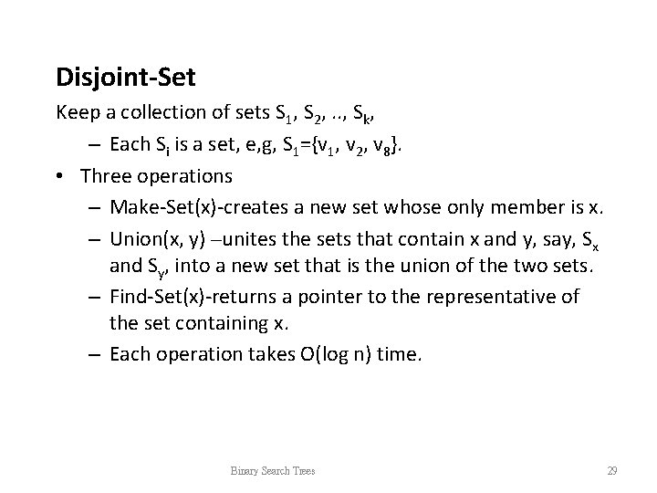
Disjoint-Set Keep a collection of sets S 1, S 2, . . , Sk, – Each Si is a set, e, g, S 1={v 1, v 2, v 8}. • Three operations – Make-Set(x)-creates a new set whose only member is x. – Union(x, y) –unites the sets that contain x and y, say, Sx and Sy, into a new set that is the union of the two sets. – Find-Set(x)-returns a pointer to the representative of the set containing x. – Each operation takes O(log n) time. Binary Search Trees 29

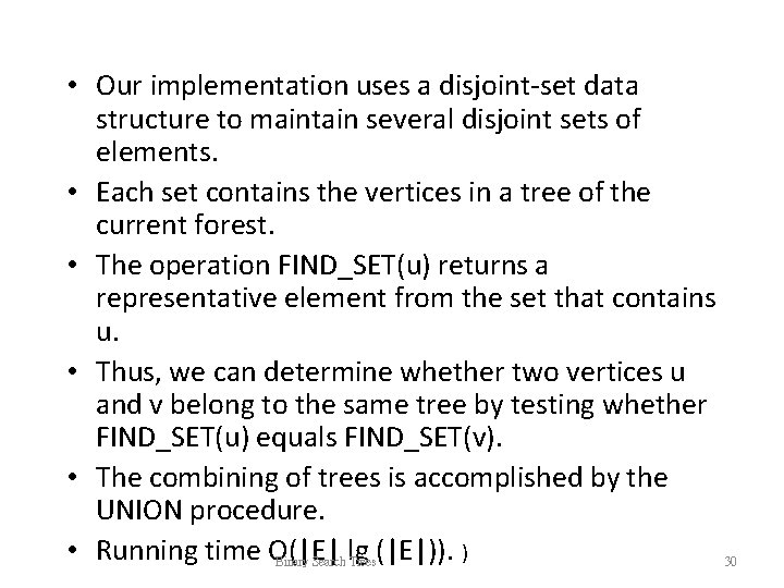
• Our implementation uses a disjoint-set data structure to maintain several disjoint sets of elements. • Each set contains the vertices in a tree of the current forest. • The operation FIND_SET(u) returns a representative element from the set that contains u. • Thus, we can determine whether two vertices u and v belong to the same tree by testing whether FIND_SET(u) equals FIND_SET(v). • The combining of trees is accomplished by the UNION procedure. • Running time O(|E| Binary Search lg Trees(|E|)). ) 30

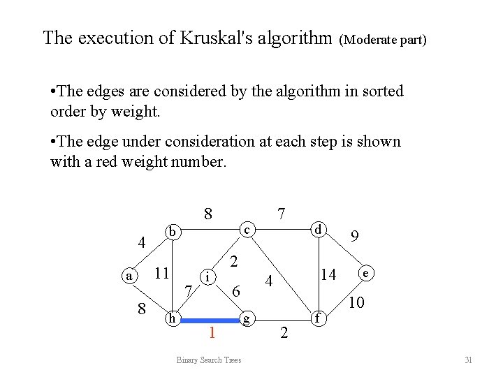
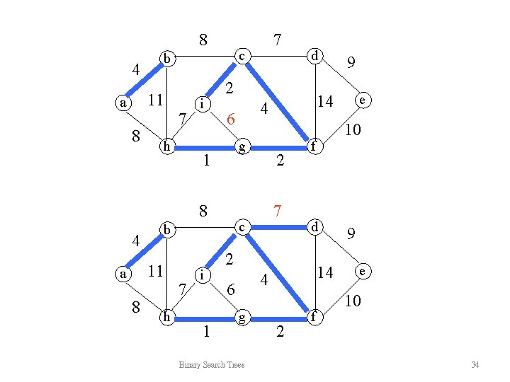
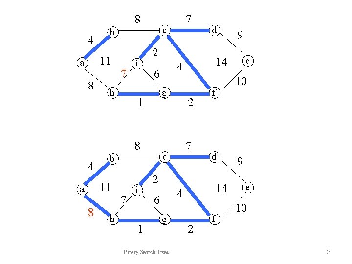
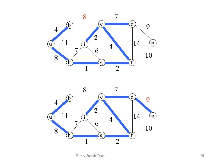
The execution of Kruskal's algorithm (Moderate part) • The edges are considered by the algorithm in sorted order by weight. • The edge under consideration at each step is shown with a red weight number. 8 4 8 c b 11 a h 7 i 7 d 2 6 1 Binary Search Trees 14 4 g 2 f 9 e 10 31

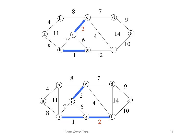
8 11 a c b 4 8 i 7 h g 1 8 h 7 i 1 2 7 c f d 2 14 4 6 g Binary Search Trees 9 e 14 4 6 b 11 a d 2 8 4 7 2 f 10 9 e 10 32

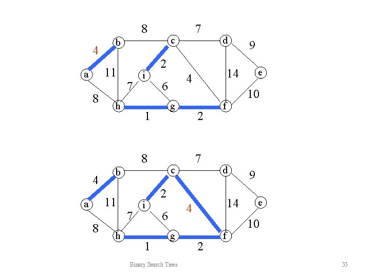
8 4 8 c b 11 a 7 h i g 1 8 h 7 i 1 2 7 c d 14 4 g Binary Search Trees e 10 f 2 6 9 14 4 6 b 11 a d 2 8 4 7 2 f 9 e 10 33

8 4 8 c b 11 a 7 h i g 1 8 h 7 i 1 2 7 c d 14 4 g Binary Search Trees e 10 f 2 6 9 14 4 6 b 11 a d 2 8 4 7 2 f 9 e 10 34

8 4 8 c b 11 a 7 h i g 1 8 h 7 i 1 2 7 c d 14 4 g Binary Search Trees e 10 f 2 6 9 14 4 6 b 11 a d 2 8 4 7 2 f 9 e 10 35

8 4 8 c b 11 a 7 h i g 1 8 h 7 i 1 2 7 c d 14 4 g Binary Search Trees e 10 f 2 6 9 14 4 6 b 11 a d 2 8 4 7 2 f 9 e 10 36

Disjoint Sets Data Structure

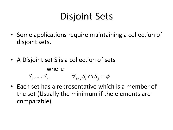
Disjoint Sets • Some applications require maintaining a collection of disjoint sets. • A Disjoint set S is a collection of sets where • Each set has a representative which is a member of the set (Usually the minimum if the elements are comparable)

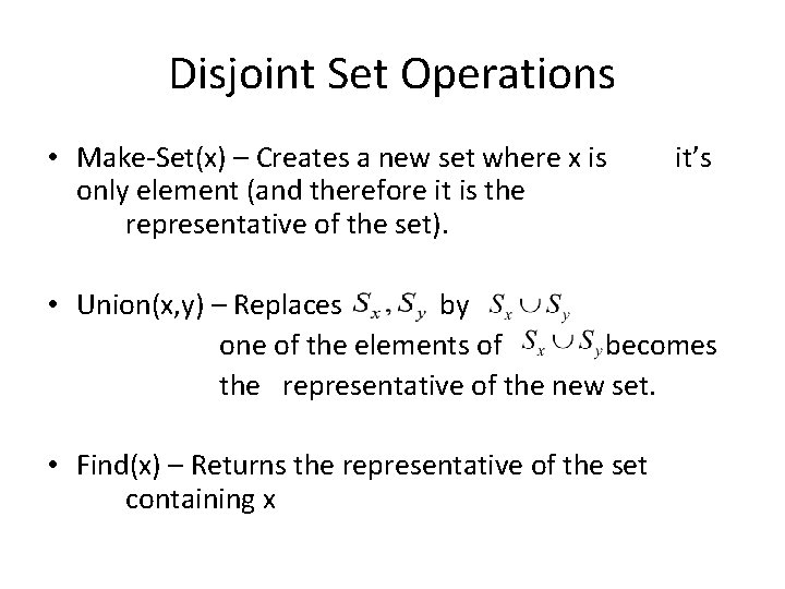
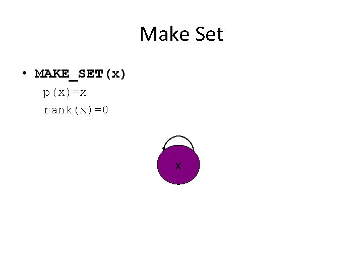
Disjoint Set Operations • Make-Set(x) – Creates a new set where x is only element (and therefore it is the representative of the set). it’s • Union(x, y) – Replaces by one of the elements of becomes the representative of the new set. • Find(x) – Returns the representative of the set containing x

Analyzing Operations • We usually analyze a sequence of m operations, of which n of them are Make_Set operations, and m is the total of Make_Set, Find, and Union operations • Each union operations decreases the number of sets in the data structure, so there can not be more than n-1 Union operations

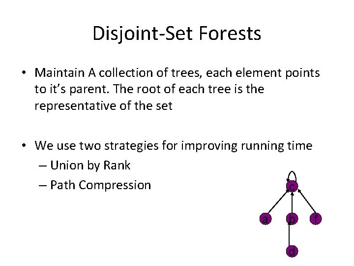
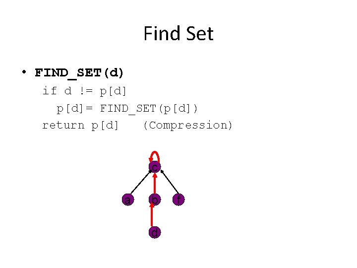
Disjoint-Set Forests • Maintain A collection of trees, each element points to it’s parent. The root of each tree is the representative of the set • We use two strategies for improving running time – Union by Rank – Path Compression c a b d f

Make Set • MAKE_SET(x) p(x)=x rank(x)=0 x

Find Set • FIND_SET(d) if d != p[d]= FIND_SET(p[d]) return p[d] (Compression) c a b d f

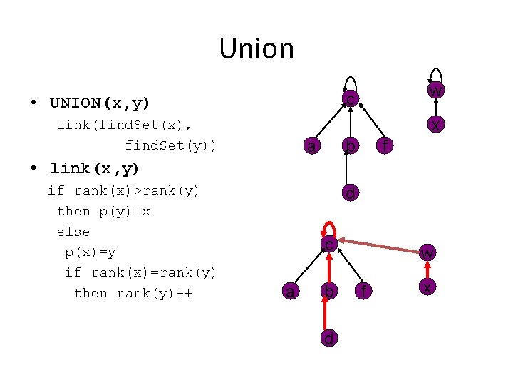
Union w c • UNION(x, y) x link(find. Set(x), find. Set(y)) a b f • link(x, y) if rank(x)>rank(y) then p(y)=x else p(x)=y if rank(x)=rank(y) then rank(y)++ d c a b d w f x

Analysis • In Union we attach a smaller tree to the larger tree, results in logarithmic depth. O(log n). – Whenever height of a tree increases by 1, size doubles. • Path compression cause a very deep tree to become very shallow

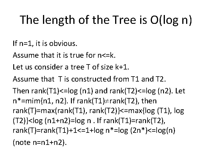
The length of the Tree is O(log n) If n=1, it is obvious. Assume that it is true for n<=k. Let us consider a tree T of size k+1. Assume that T is constructed from T 1 and T 2. Then rank(T 1)<=log (n 1) and rank(T 2)<=log (n 2). Let n*=mim{n 1, n 2}. If rank(T 1) rank(T 2), then rank(T)=max(rank(T 1), rank(T 2)}<=max{log (T 1), log (T 2)}<log (n 1+n 2)=log n. If rank(T 1)=rank(T 2), rank(T)=rank(T 1)+1<=1+log n*=log (2 n*)<=log(n) (note n=n 1+n 2).