Minimum Spanning Tree A Minimum Spanning Tree MST

Minimum Spanning Tree • A Minimum Spanning Tree (MST) is a subgraph of an undirected graph such that the subgraph spans (includes) all nodes, is connected, is acyclic, and has minimum total edge weight

Algorithm Characteristics • Both Prim’s and Kruskal’s Algorithms work with undirected graphs • Both work with weighted and unweighted graphs but are more interesting when edges are weighted • Both are greedy algorithms that produce optimal solutions

Prim’s Algorithm • Similar to Dijkstra’s Algorithm except that distance records edge weights, not path lengths

Walk-Through 2 F 10 C 7 A 4 8 4 B 9 H Initialize array 3 3 G D 10 25 7 E d A F B F C F D F E F F F G F H F 3 18 2 in Tree? pv v

2 F 10 A 7 B 9 H G D 10 25 7 in Tree? dv pv T 0 A 18 2 3 C 3 4 8 4 Start with any node, say D 3 E B C D E F G H

Update distances of adjacent, unselected nodes 2 F 10 A 7 4 8 4 B 9 H C 3 3 G 25 E pv 3 D 0 E 25 D F 18 D G 2 D 3 D 10 7 dv A 18 2 in Tree? B C D H T

Select node with minimum distance 2 F 10 A 3 7 4 H 3 G 25 7 pv 3 D 0 E 25 D F 18 D 2 D A D 10 2 dv B 18 B 9 tree? 3 4 8 C E C D G H T T

Update distances of adjacent, unselected nodes 2 F 10 A 3 7 4 H 3 G 25 7 pv 3 D 0 E 7 G F 18 D 2 D 3 G A D 10 2 dv B 18 B 9 tree? 3 4 8 C E C D G H T T

Select node with minimum distance 2 F 10 A 3 7 4 H 3 D 10 25 2 G 7 dv pv C T 3 D D T 0 E 7 G F 18 D 2 D 3 G B 18 B 9 in tree? A 3 4 8 C E G H T

Update distances of adjacent, unselected nodes 2 F 10 A 3 7 4 H 25 2 3 D 10 G 7 E dv pv 4 C A B 18 B 9 in tree? 3 4 8 C C T 3 D D T 0 E 7 G F 3 C 2 D 3 G G H T

Select node with minimum distance 2 F 10 A 3 7 4 H 25 2 3 D 10 G 7 E dv pv 4 C A B 18 B 9 in tree? 3 4 8 C C T 3 D D T 0 7 G E F T 3 C G T 2 D 3 G H

Update distances of adjacent, unselected nodes 2 F 10 A 3 7 4 H 18 B 9 D 10 25 2 3 G in tree? 3 4 8 C 7 E dv pv A 10 F B 4 C C T 3 D D T 0 2 F E F T 3 C G T 2 D 3 G H

Select node with minimum distance 2 F 10 A 3 7 4 H 18 B 9 D 10 25 2 3 G In Tree? 3 4 8 C 7 E dv pv A 10 F B 4 C C T 3 D D T 0 E T 2 F F T 3 C G T 2 D 3 G H

Update distances of adjacent, unselected nodes 2 F 10 A 3 7 4 H 18 B 9 D 10 25 2 3 G in Tree? 3 4 8 C 7 E dv pv A 10 F B 4 C C T 3 D D T 0 E T 2 F F T 3 C G T 2 D 3 G H Table entries unchanged

Select node with minimum distance 2 F 10 A 3 7 4 H 18 B 9 D 10 25 2 3 G in Tree? dv pv A 10 F B 4 C 3 4 8 C 7 E C T 3 D D T 0 E T 2 F F T 3 C G T 2 D H T 3 G

Update distances of adjacent, unselected nodes 2 F 10 A 3 7 4 H 18 B 9 D 10 25 2 3 G in Tree? dv pv A 4 H B 4 C 3 4 8 C 7 E C T 3 D D T 0 E T 2 F F T 3 C G T 2 D H T 3 G

Select node with minimum distance 2 F 10 A 3 7 4 18 B 9 H 3 4 8 G 25 7 A D 10 2 3 C E in Tree? dv pv T 4 H 4 C B C T 3 D D T 0 E T 2 F F T 3 C G T 2 D H T 3 G

Update distances of adjacent, unselected nodes 2 F 10 A 3 7 4 H 3 D 10 25 2 G 7 in Tree? dv pv T 4 H 4 C B 18 B 9 A 3 4 8 C E C T 3 D D T 0 E T 2 F F T 3 C G T 2 D H T 3 G Table entries unchanged

Select node with minimum distance 2 F 10 A 3 7 4 18 B 9 H 3 4 8 D 10 25 2 3 C G 7 E in Tree? dv pv A T 4 H B T 4 C C T 3 D D T 0 E T 2 F F T 3 C G T 2 D H T 3 G

Cost of Minimum Spanning Tree = dv = 21 2 3 F A C B H D 2 3 G dv pv A T 4 H B T 4 C C T 3 D D T 0 E T 2 F F T 3 C G T 2 D H T 3 G 3 4 4 in Tree? E Done

Kruskal’s Algorithm Work with edges, rather than nodes Two steps: – Sort edges by increasing edge weight – Select the first |V| – 1 edges that do not generate a cycle

Walk-Through F 1 A 4 H 6 B 4 D 4 1 2 3 C 3 4 8 5 Consider an undirected, weight graph 3 G 3 E

F 1 A 4 H 6 B 4 D 4 1 2 3 C 3 4 8 5 Sort the edges by increasing edge weight 3 G 3 E edge dv (A, F) 1 (B, E) 4 (D, E) 1 (B, F) 4 (D, G) 2 (B, H) 4 (E, G) 3 (A, H) 5 (C, D) 3 (D, F) 6 (G, H) 3 (A, B) 8 (C, F) 3 (B, C) 4

Select first |V|– 1 edges which do not generate a cycle F 1 A 3 4 6 B 5 4 H 3 4 8 D 4 1 2 3 C G 3 E edge dv (B, E) 4 (B, F) 4 2 (B, H) 4 (E, G) 3 (A, H) 5 (C, D) 3 (D, F) 6 (G, H) 3 (A, B) 8 (C, F) 3 (B, C) 4 edge dv (A, F) 1 (D, E) 1 (D, G)

Select first |V|– 1 edges which do not generate a cycle F 1 A 3 4 5 6 B 4 H 3 4 8 D 4 1 2 3 C G 3 E edge dv (B, E) 4 1 (B, F) 4 (D, G) 2 (B, H) 4 (E, G) 3 (A, H) 5 (C, D) 3 (D, F) 6 (G, H) 3 (A, B) 8 (C, F) 3 (B, C) 4 edge dv (A, F) 1 (D, E)

Select first |V|– 1 edges which do not generate a cycle F 1 A 3 4 5 6 B 4 H 3 4 8 D 4 1 2 3 C G 3 E edge dv (B, E) 4 1 (B, F) 4 (D, G) 2 (B, H) 4 (E, G) 3 (A, H) 5 (C, D) 3 (D, F) 6 (G, H) 3 (A, B) 8 (C, F) 3 (B, C) 4 edge dv (A, F) 1 (D, E) Accepting edge (E, G) would create a cycle

Select first |V|– 1 edges which do not generate a cycle 3 F 1 A 4 5 3 4 8 6 B 4 D 4 H 1 2 3 C G 3 E edge dv (B, E) 4 1 (B, F) 4 (D, G) 2 (B, H) 4 (E, G) 3 (A, H) 5 (C, D) 3 (D, F) 6 (G, H) 3 (A, B) 8 (C, F) 3 (B, C) 4 edge dv (A, F) 1 (D, E)

Select first |V|– 1 edges which do not generate a cycle F 1 A 3 4 5 6 B 4 H 3 4 8 D 4 1 2 3 C G 3 E edge dv (B, E) 4 1 (B, F) 4 (D, G) 2 (B, H) 4 (E, G) 3 (A, H) 5 (C, D) 3 (D, F) 6 (G, H) 3 (A, B) 8 (C, F) 3 (B, C) 4 edge dv (A, F) 1 (D, E)

Select first |V|– 1 edges which do not generate a cycle F 1 A 3 4 5 6 B 4 H 3 4 8 D 4 1 2 3 C G 3 E edge dv (B, E) 4 1 (B, F) 4 (D, G) 2 (B, H) 4 (E, G) 3 (A, H) 5 (C, D) 3 (D, F) 6 (G, H) 3 (A, B) 8 (C, F) 3 (B, C) 4 edge dv (A, F) 1 (D, E)

Select first |V|– 1 edges which do not generate a cycle F 1 A 3 4 5 6 B 4 H 3 4 8 D 4 1 2 3 C G 3 E edge dv (B, E) 4 2 (B, F) 4 (E, G) 3 (B, H) 4 (C, D) 3 (A, H) 5 (G, H) 3 (D, F) 6 (C, F) 3 (A, B) 8 (B, C) 4 edge dv (D, E) 1 (D, G)

Select first |V|– 1 edges which do not generate a cycle 3 F A C 3 4 B H 2 3 G D 1 E Done Total Cost = dv = 17

Euler Paths and Circuits • The Seven bridges of Königsberg. Can you take a walk and visit all bridges exactly once? You don’t have to end up where you began? • Map physical situation into a graph. Euler 1735. Beginning of graph theory. • Draw the corresponding graph in which nodes represent land areas and arcs represent bridges connecting the land areas. . C D A B

Euler Paths and Circuits • • • The Seven bridges of Königsberg. Can you take a walk and visit all bridges exactly once? You don’t have to end up where you began. Map physical situation into a graph. Swiss Leonhard Euler 1735 (contemporary of Ben Franklin). Beginning of graph theory. Interesting presentation on Euler https: //www. youtube. com/watch? v=h-DV 26 x 6 n_Q C c D A B d a b

Euler Paths and Circuits • An Euler path is a path using every edge of the graph G exactly once. • An Euler circuit is an Euler path that returns to its start. C Does this graph have an Euler circuit? No. D A B

Necessary and Sufficient Conditions • How about multigraphs (permitted to have multiple edges between same end nodes)? • A connected multigraph has a Euler circuit iff each of its vertices has an even degree. • A connected multigraph has a Euler path but not an Euler circuit iff it has exactly two vertices of odd degree.

Example • Which of the following graphs has an Euler circuit? a b a e d b a b c c d e

Example • Which of the following graphs has an Euler circuit? a b a e d b a b c c d e c yes (a, e, c, d, e, b, a) d no no e

Example • Which of the following graphs has an Euler path? a b a e d b a b c c d e c d yes no (a, e, c, d, e, b, a ) yes (a, c, d, e, b, d, a, b) e

Euler Circuit in Directed Graphs

Euler Path in Directed Graphs NO (a, g, c, b, g, e, d, f, a) (c, a, b, c, d, b)

Real Life Applications of Eulerian Circuits/Tours • Snow removal, inspecting railroad tracks, Postal Route, collecting garbage, checking parking meters • May need to “Eulerize” – add arcs to make Eulerian • DNA sequencing and fragment assembly • Designs - Kolam

Hamilton Paths and Circuits • A Hamilton path in a graph G is a path which visits every vertex in G exactly once. • A Hamilton circuit is a Hamilton path that returns to its start.

Dodecahedron is composed of twelve regular pentagons. Can you find a path which visits all vertices? Can you draw it as a graph?

Hamilton Circuits Dodecahedron puzzle equivalent graph Is there a circuit in this graph that passes through each vertex exactly once?

Hamilton Circuits Yes; this is a circuit that passes through each vertex exactly once.

Finding Hamilton Circuits Which of these three figures has a Hamilton circuit? Or, if no Hamilton circuit, a Hamilton path?

Finding Hamilton Circuits • G 1 has a Hamilton circuit: a, b, c, d, e, a • G 2 does not have a Hamilton circuit, but does have a Hamilton path: a, b, c, d • G 3 has neither.

Finding Hamilton Circuits • Unlike the Euler circuit problem, finding Hamilton circuits is hard. • There is no simple set of necessary and sufficient conditions, and no simple algorithm.

Real Life applications? • Anything where you have to visit all locations: – Pizza delivery – Mail delivery – Garbage pickup – Bus service/limousine service – Reading gas meters – Traveling Salesman Problem – finding a Hamilton circuit in a complete graph such that the total weight of its edges is minimal

Edge types • • If we do a depth first search on a directed graph, we may get a forest rather than just a tree. We get forward (to a descendant (but not a child)), back (to an ancestor), and cross edges (to unrelated node). For the graph which follows show the different types of edges. Start at B

Edge types • • • Edge types depend on type of graph and type of traversal. If we do a depth first search on a directed graph, we may get a forest rather than just a tree. The edges we selected are termed tree edges We get forward (bold), back (to an ancestor), and cross edges (to unrelated node). For the graph which follows show the different types of edges. Start at B, Then H then G.

“Shaking down the tree” . These labels can be helpful in other algorithms as they give structure to the graph.

Finding Strong Components First do a depth-first search, numbering nodes in postorder. When tracing on paper, I find it easiest to highlight the edges so I can keep the traversal straight. We may have to restart several times. In this case, we start at A, then C (picking a new starting place by alphabetical ordering, just to be consistent). We mark them as visited when we first enter dfs. Post, but we number after visiting all children. // Visits all nodes in depth first order, but number AFTER visiting kids dfs. Post (node) { node. visited = true; for each successor of node if successor is unvisited dfs. Post(successor) node. number = dfs++; // dfs is a class variable }

Start at A

Next start at C - considering unvisited nodes in alphabetical order for those obsessive compulsive types (you know who you are)

Depth first postorder numbering

Reverse all edges. Clear visited flags. Do a depth first search marking nodes as visited. Always starting a tree at the highest numbered (unvisited)node.

Reverse all edges. Clear visited flags. Do a depth first search marking nodes as visited. Always starting a tree at the highest numbered node which hasn’t been visited.

• Each tree of the forest of this second depth first search is a strongly connected component. – Start at C: 15 {ECNOIKH} – Continue at J: 11 {J} – Continue at F: 10 {FM} – Continue at A: 5 {ALDB} – Continue at G: 1 {G}

Maximum Network Flow Problem • How can we maximize the flow in a network from a source or set of sources to a destination of set of destinations? • The problem reportedly rose to prominence in relation to the rail networks of the Soviet Union, during the 1950's. The US wanted to know how quickly the Soviet Union could get supplies through its rail network to its satellite states in Eastern Europe. • In addition, the US wanted to know which rails it could destroy most easily to cut off the satellite states from the rest of the Soviet Union. – It turned out that these two problems were closely related, and that solving the max flow problem also solves the min cut problem of figuring out the cheapest way to cut off the Soviet Union from its satellites. • The first efficient algorithm for finding the maximum flow was conceived by two Computer Scientists, named Ford and Fulkerson. The algorithm was subsequently named the Ford-Fulkerson algorithm, and is one of the more famous algorithms in computer science. Source: lbackstrom, The Importance of Algorithms, at www. topcoder. com

Network Flow • A Network is a directed graph G • Edges represent pipes that carry flow • Each edge <u, v> has a maximum capacity c<u, v> • A source node s in which flow arrives • A sink node t out which flow leaves Goal: Max Flow

Network Flow • The network flow problem is as follows: – Given a connected directed graph G • with non-negative integer weights, • (where each edge stands for the capacity of that edge), – 2 different vertices, s and t, called the source and the sink, • such that the source only has out-edges and the sink only has in-edges, – Find the maximum amount of some commodity that can flow through the network from source to sink. 12 a b 16 s 13 4 10 9 20 7 t 4 c 14 d Each edge stands for the capacity of that edge.

Network Flow • One way to imagine the situation is imagining each edge is a way of transporting students between nodes. – The source is where the students are now. The sink is where they want to be. – Each edge weight specifies the maximal number of students that can be transported – Given that information, what is the most students that can be moved from the source to the sink? 12 a b 16 s 13 4 10 9 20 7 t 4 c 14 d Each edge stands for the capacity of that edge.

Network Flow 12 a b 16 s 4 10 9 20 14 b 12/16 t 4 c 12/12 19/20 0/9 7 13 a d This graph contains the capacities of each edge in the graph. s 0/4 0/10 t 7/7 11/13 4/4 c 11/14 d Here is an example of a flow in the graph. • The flow of the network is defined as the flow from the source, or into the sink. • For the situation above, the network flow is 23.

12 a b 16 s 4 10 9 20 7 12/16 t 4 14 b 19/20 0/9 13 c 12/12 a d s 0/4 0/10 t 7/7 11/13 4/4 c capacities 11/14 d flow • The Conservation Rule: – In order for the assignment of flows to be valid, we must have the sum of flow coming into a vertex equal to the flow coming out of a vertex, for each vertex in the graph except the source and the sink. • The Capacity Rule: – Also, each flow must be less than or equal to the capacity of the edge. • The flow of the network is defined as the flow from the source, or into the sink. – For the situation above, the network flow is 23.

Network Flow • In order to determine the maximum flow of a network, we will use the following terms: – Residual capacity – is simply an edge’s unused capacity. • Initially none of the capacities will have been used, so all of the residual capacities will be just the original capacity. a 0/12 b 0/16 0/20 0/9 s 0/4 0/10 t 0/7 0/4 0/13 c 0/14 d Using the notation: used / capacity. Residual Capacity: capacity - used.

Network Flow – Residual capacity of a path – the minimum of the residual capacities of the edges on that path, which will end up being the max excess flow we can push down that path. – Augmenting path – defined as one where you have a path from the source to the sink where every edge has a nonzero residual capacity. a 0/12 b 0/16 0/20 0/9 s 0/4 0/10 t 0/7 0/4 0/13 c 0/14 d Using the notation: used / unused. Residual Capacity: unused - used.

1 1

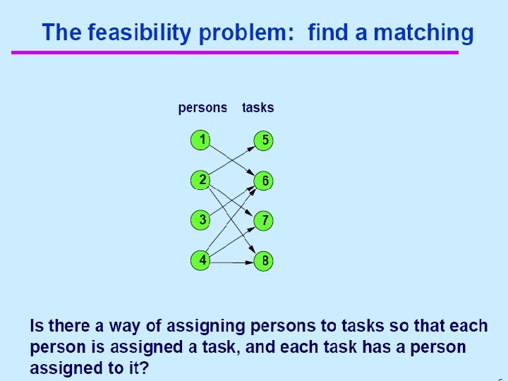
m A n B o C p D q How could network flow solve this matching problem?

m A n B o C p D q Note: Every edge has capacity 1.

Idea, find one path at a time.

Can we do better?

We could start over and hope to make better choices. What about trying to augment existing paths? We can go backwards on an arc with forward flow.

The arcs that we went backward on, now have zero flow. The pictures is as below

Ford-Fulkerson Algorithm While there exists an augmenting path Add the appropriate flow to that augmenting path • Arbitrarily choose the augmenting path s, c, d, t in the graph below: – And add the flow to that path. a 0/12 b 0/16 0/20 0/9 s 0/4 0/10 t 0/7 4/4 0/4 4/13 0/13 c 4/14 0/14 d ◦ Residual capacity of a path – the minimum of the residual capacities of the edges on that path. ◦ 4 in this case, which is the limiting factor for this path’s flow.

Ford-Fulkerson Algorithm While there exists an augmenting path Add the appropriate flow to that augmenting path • Choose another augmenting path (one where you have a path from the source to the sink where every edge has a nonzero residual capacity. ) – s, a, b, t a 12/12 0/12 b 12/16 0/16 12/20 0/9 s 4/13 0/4 0/10 t 0/7 4/4 c 4/14 d ◦ Residual capacity of a path – the minimum of the residual capacities of the edges on that path. ◦ 12 in this case, which is the limiting factor for this path’s flow.

Ford-Fulkerson Algorithm While there exists an augmenting path Add the appropriate flow to that augmenting path • Choose another augmenting path (one where you have a path from the source to the sink where every edge has a nonzero residual capacity. ) – s, c, d, b, t a 12/12 b 12/20 19/20 12/16 0/9 s 0/4 4/13 11/13 0/10 t 0/7 7/7 4/4 c 4/14 11/14 d ◦ Residual capacity of a path – the minimum of the residual capacities of the edges on that path. ◦ 7 in this case, which is the limiting factor for this path’s flow.

Ford-Fulkerson Algorithm While there exists an augmenting path Add the appropriate flow to that augmenting path • Are there any more augmenting paths? – No! We’re done – The maximum flow = 19 + 4 = 23 a 12/12 b 12/16 19/20 0/9 s 0/4 0/10 t 7/7 11/13 4/4 c 11/14 d

What if we picked path s-a-d-t? We need to allow the algorithm to change its mind. To do so, in the residual graph we allow an edge going backwards on any path with positive flow. In this example, we could go backwards along path from d to a.

What if you were really unlucky? How can you avoid?

Ford-Fulkerson Algorithm Runtime While there exists an augmenting path Add the appropriate flow to that augmenting path • We can check the existence of an augmenting path by doing a graph traversal on the network (with all full capacity edges removed. ) – This graph, a subgraph with all edges of full capacity removed is called a residual graph. • It is difficult to analyze the true running time of this algorithm because it is unclear exactly how many augmenting paths can be found in an arbitrary flow network. – In the worst case, each augmenting path adds 1 to the flow of a network, and each search for an augmenting path takes O(E) time, where E is the number of edges in the graph. – Thus, at worst-case, the algorithm takes O(|f|E) time, where |f| is the maximal flow of the network.

Edmonds-Karp Algorithm • This algorithm is a variation on the Ford. Fulkerson method which is intended to increase the speed of the first algorithm. • The idea is to try to choose good augmenting paths. – In this algorithm, the augmenting path suggested is the augmenting path with the minimal number of edges.