MiniExcursion 3 The Mathematics of Population Growth Pages
- Slides: 32

Mini-Excursion 3 The Mathematics of Population Growth Pages 474 -491 Copyright © 2010 Pearson Education, Inc. Excursions in Modern Mathematics, 7 e: 10. 6 - 1

Continuous vs. Discrete Growth • Population growth is a time-dependent process. • Discrete growth occurs when there are gaps in the growth times. • Continuous growth occurs without gaps between growth times. Copyright © 2010 Pearson Education, Inc. Excursions in Modern Mathematics, 7 e: 10. 6 - 2

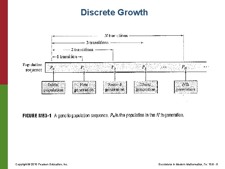
Discrete Growth • During discrete population growth, there will be sudden changes in the population called a transition. • A mathematical model of population growth defines the transition rules in the form of an equation. Copyright © 2010 Pearson Education, Inc. Excursions in Modern Mathematics, 7 e: 10. 6 - 3

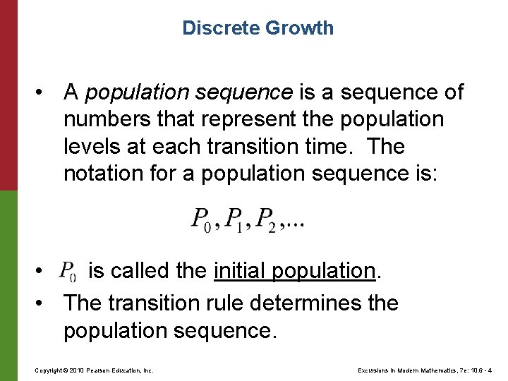
Discrete Growth • A population sequence is a sequence of numbers that represent the population levels at each transition time. The notation for a population sequence is: • is called the initial population. • The transition rule determines the population sequence. Copyright © 2010 Pearson Education, Inc. Excursions in Modern Mathematics, 7 e: 10. 6 - 4

Discrete Growth Copyright © 2010 Pearson Education, Inc. Excursions in Modern Mathematics, 7 e: 10. 6 - 5

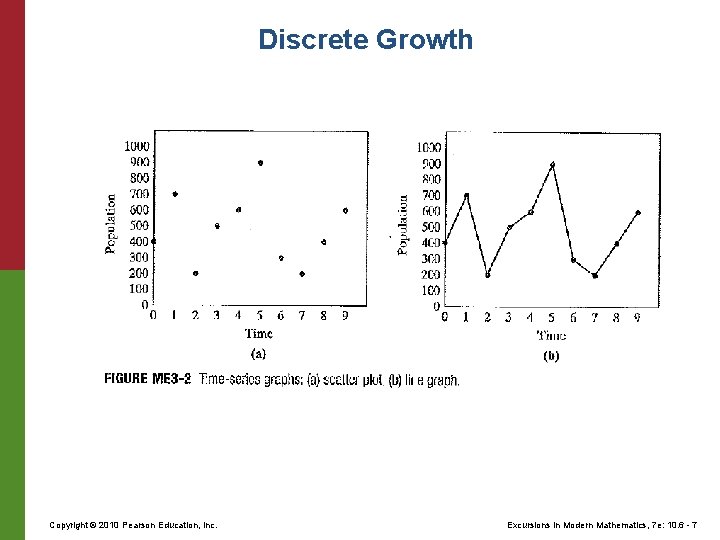
Discrete Growth • A time-series graph shows the time of each transition on the horizontal axis and the size of the population on the vertical axis. Copyright © 2010 Pearson Education, Inc. Excursions in Modern Mathematics, 7 e: 10. 6 - 6

Discrete Growth Copyright © 2010 Pearson Education, Inc. Excursions in Modern Mathematics, 7 e: 10. 6 - 7

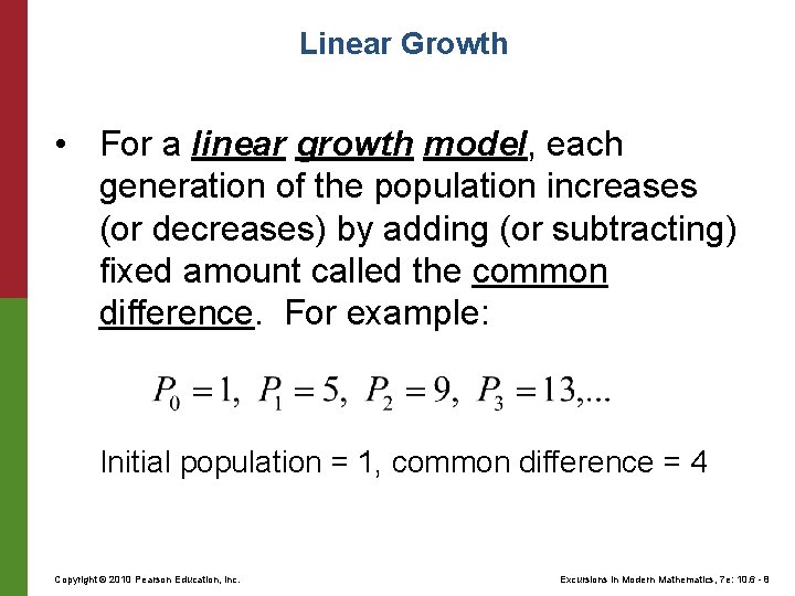
Linear Growth • For a linear growth model, each generation of the population increases (or decreases) by adding (or subtracting) fixed amount called the common difference. For example: Initial population = 1, common difference = 4 Copyright © 2010 Pearson Education, Inc. Excursions in Modern Mathematics, 7 e: 10. 6 - 8

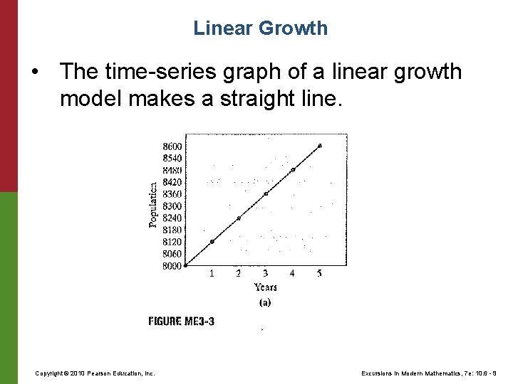
Linear Growth • The time-series graph of a linear growth model makes a straight line. Copyright © 2010 Pearson Education, Inc. Excursions in Modern Mathematics, 7 e: 10. 6 - 9

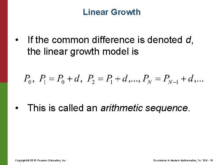
Linear Growth • If the common difference is denoted d, the linear growth model is • This is called an arithmetic sequence. Copyright © 2010 Pearson Education, Inc. Excursions in Modern Mathematics, 7 e: 10. 6 - 10

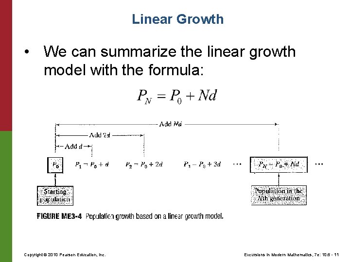
Linear Growth • We can summarize the linear growth model with the formula: Copyright © 2010 Pearson Education, Inc. Excursions in Modern Mathematics, 7 e: 10. 6 - 11

Example • Problem 4 on page 488 Copyright © 2010 Pearson Education, Inc. Excursions in Modern Mathematics, 7 e: 10. 6 - 12

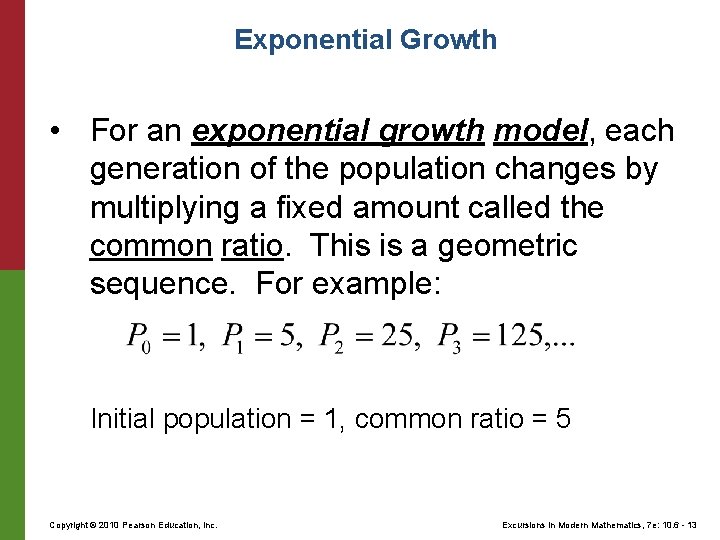
Exponential Growth • For an exponential growth model, each generation of the population changes by multiplying a fixed amount called the common ratio. This is a geometric sequence. For example: Initial population = 1, common ratio = 5 Copyright © 2010 Pearson Education, Inc. Excursions in Modern Mathematics, 7 e: 10. 6 - 13

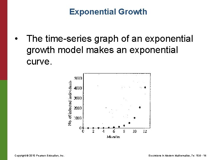
Exponential Growth • The time-series graph of an exponential growth model makes an exponential curve. Copyright © 2010 Pearson Education, Inc. Excursions in Modern Mathematics, 7 e: 10. 6 - 14

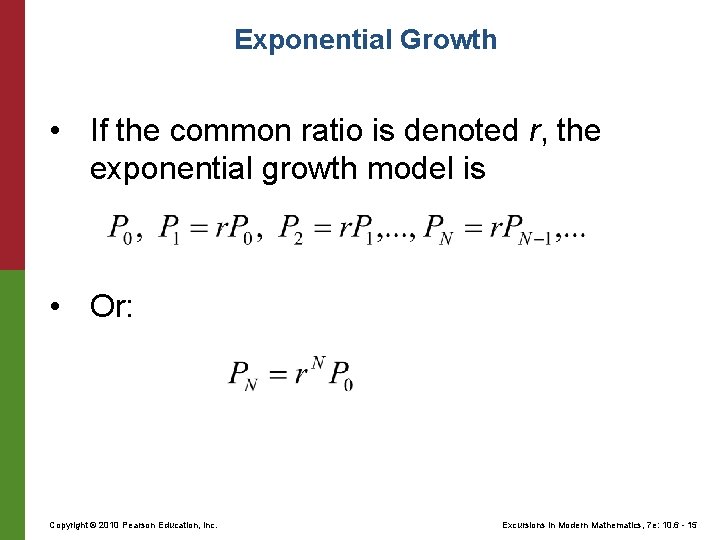
Exponential Growth • If the common ratio is denoted r, the exponential growth model is • Or: Copyright © 2010 Pearson Education, Inc. Excursions in Modern Mathematics, 7 e: 10. 6 - 15

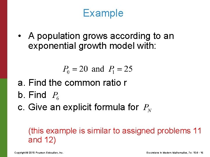
Example • A population grows according to an exponential growth model with: a. Find the common ratio r b. Find c. Give an explicit formula for (this example is similar to assigned problems 11 and 12) Copyright © 2010 Pearson Education, Inc. Excursions in Modern Mathematics, 7 e: 10. 6 - 16

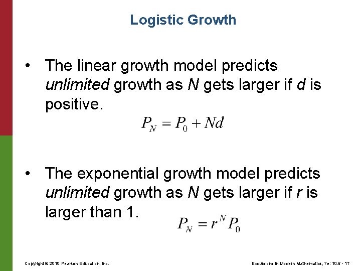
Logistic Growth • The linear growth model predicts unlimited growth as N gets larger if d is positive. • The exponential growth model predicts unlimited growth as N gets larger if r is larger than 1. Copyright © 2010 Pearson Education, Inc. Excursions in Modern Mathematics, 7 e: 10. 6 - 17

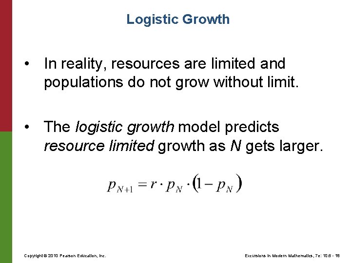
Logistic Growth • In reality, resources are limited and populations do not grow without limit. • The logistic growth model predicts resource limited growth as N gets larger. Copyright © 2010 Pearson Education, Inc. Excursions in Modern Mathematics, 7 e: 10. 6 - 18

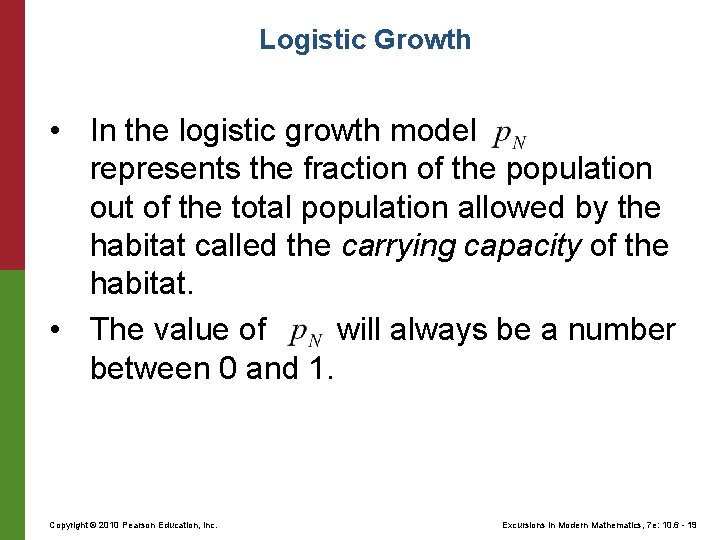
Logistic Growth • In the logistic growth model represents the fraction of the population out of the total population allowed by the habitat called the carrying capacity of the habitat. • The value of will always be a number between 0 and 1. Copyright © 2010 Pearson Education, Inc. Excursions in Modern Mathematics, 7 e: 10. 6 - 19

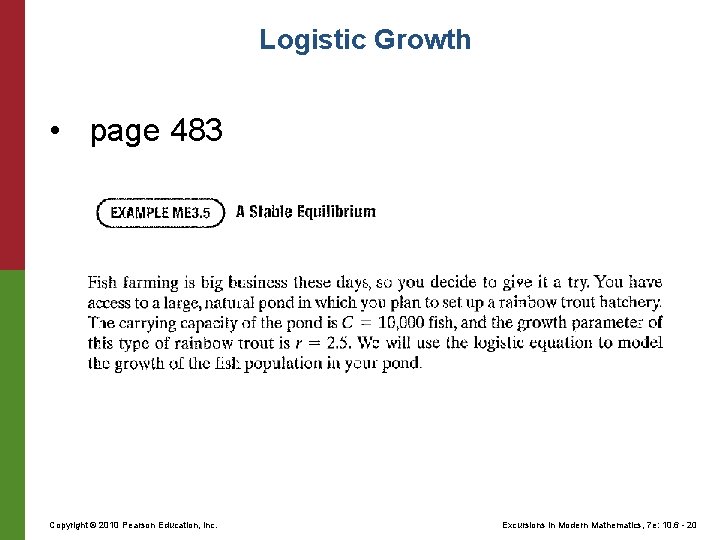
Logistic Growth • page 483 Copyright © 2010 Pearson Education, Inc. Excursions in Modern Mathematics, 7 e: 10. 6 - 20

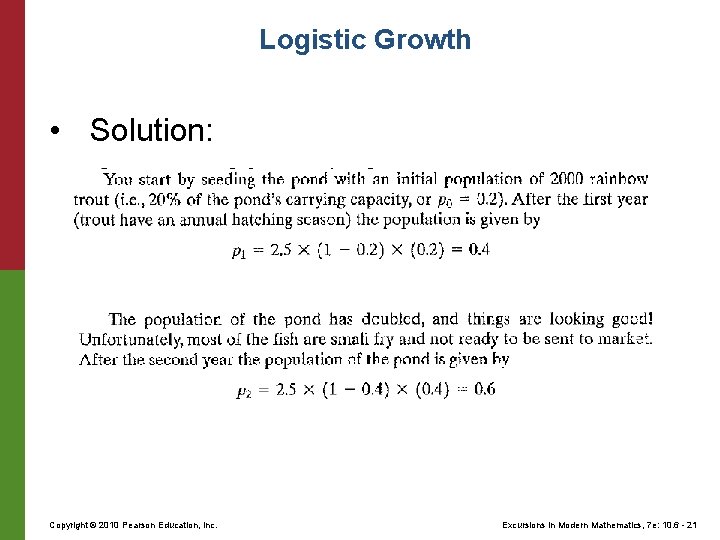
Logistic Growth • Solution: Copyright © 2010 Pearson Education, Inc. Excursions in Modern Mathematics, 7 e: 10. 6 - 21

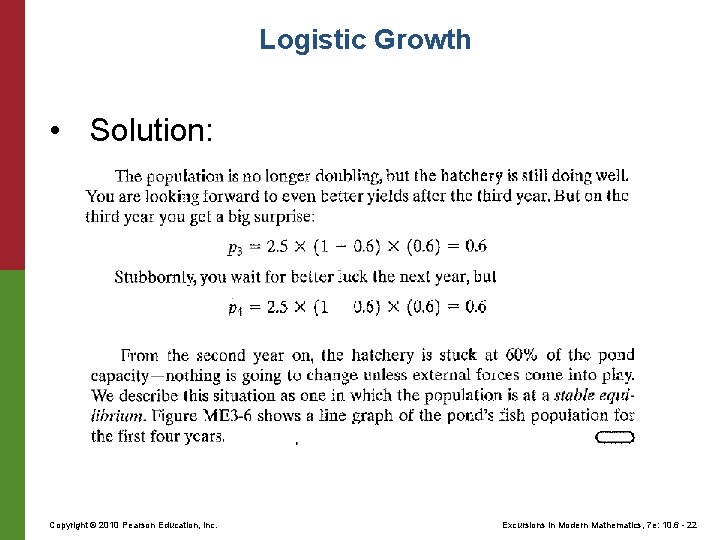
Logistic Growth • Solution: Copyright © 2010 Pearson Education, Inc. Excursions in Modern Mathematics, 7 e: 10. 6 - 22

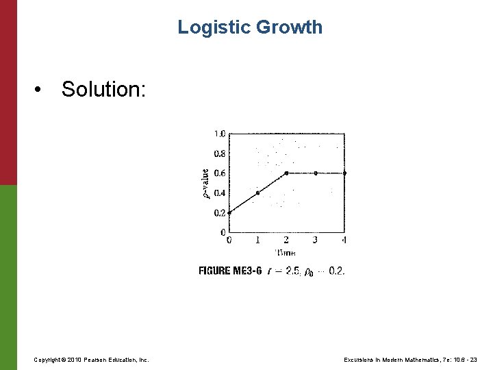
Logistic Growth • Solution: Copyright © 2010 Pearson Education, Inc. Excursions in Modern Mathematics, 7 e: 10. 6 - 23

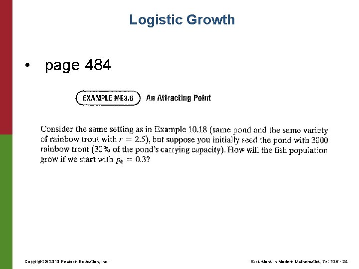
Logistic Growth • page 484 Copyright © 2010 Pearson Education, Inc. Excursions in Modern Mathematics, 7 e: 10. 6 - 24

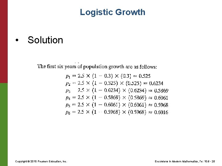
Logistic Growth • Solution Copyright © 2010 Pearson Education, Inc. Excursions in Modern Mathematics, 7 e: 10. 6 - 25

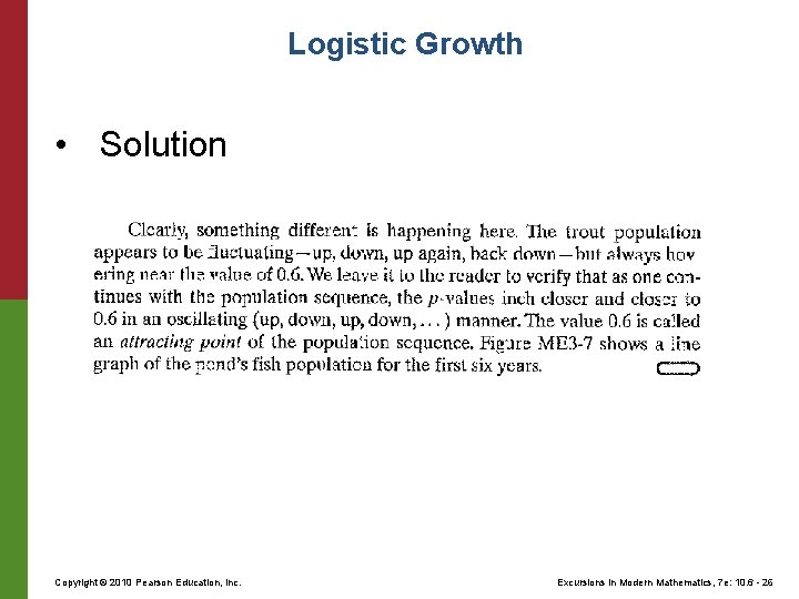
Logistic Growth • Solution Copyright © 2010 Pearson Education, Inc. Excursions in Modern Mathematics, 7 e: 10. 6 - 26

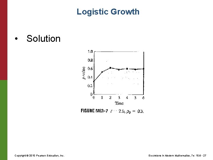
Logistic Growth • Solution Copyright © 2010 Pearson Education, Inc. Excursions in Modern Mathematics, 7 e: 10. 6 - 27

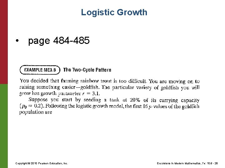
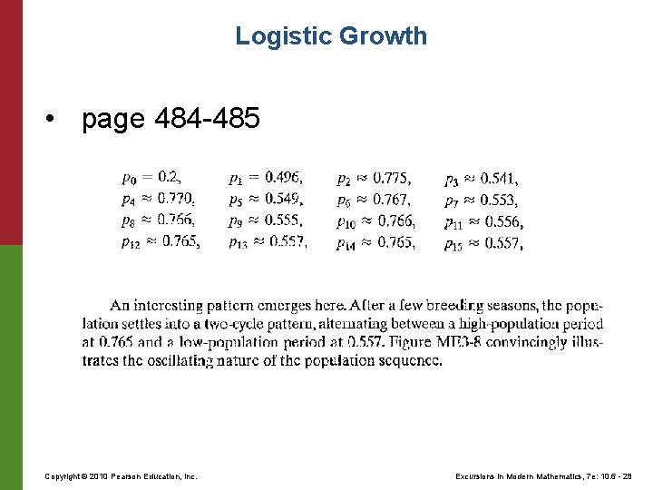
Logistic Growth • page 484 -485 Copyright © 2010 Pearson Education, Inc. Excursions in Modern Mathematics, 7 e: 10. 6 - 28

Logistic Growth • page 484 -485 Copyright © 2010 Pearson Education, Inc. Excursions in Modern Mathematics, 7 e: 10. 6 - 29

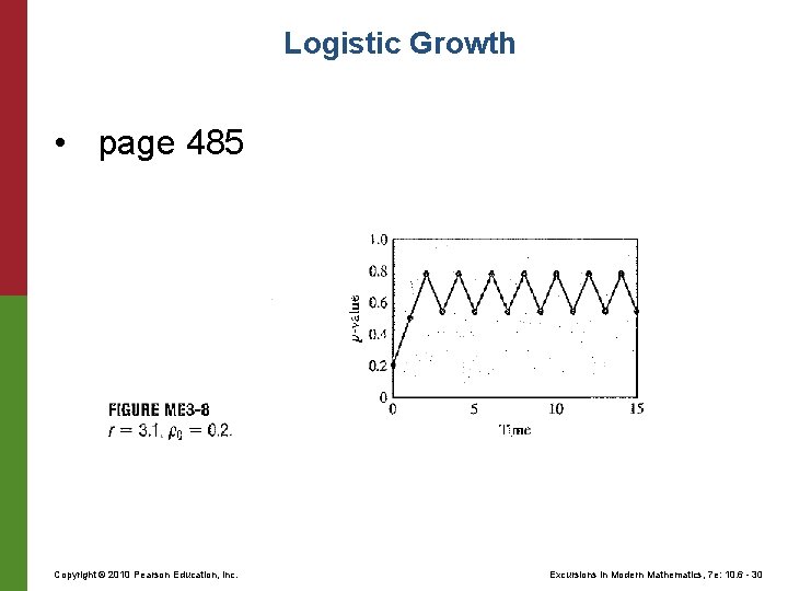
Logistic Growth • page 485 Copyright © 2010 Pearson Education, Inc. Excursions in Modern Mathematics, 7 e: 10. 6 - 30

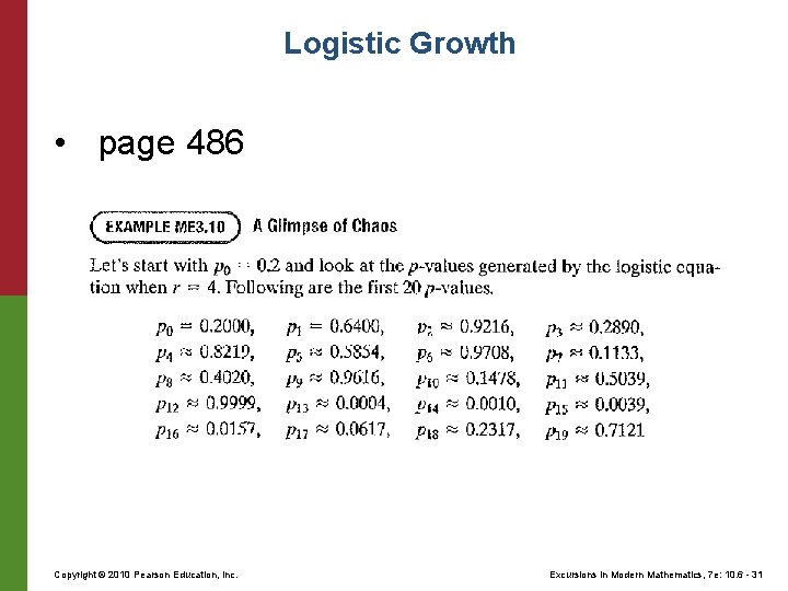
Logistic Growth • page 486 Copyright © 2010 Pearson Education, Inc. Excursions in Modern Mathematics, 7 e: 10. 6 - 31

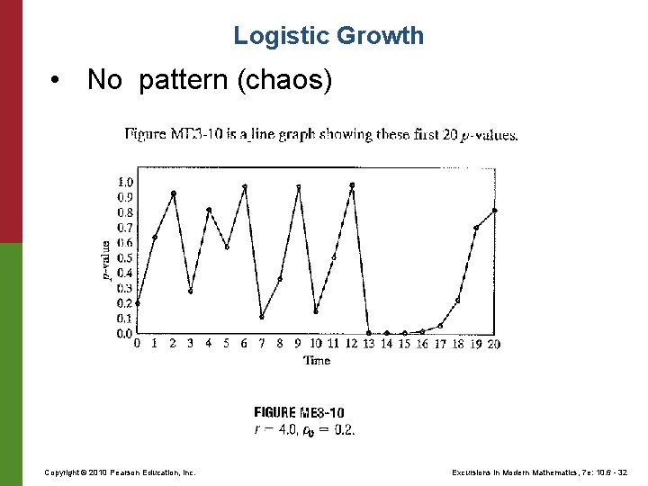
Logistic Growth • No pattern (chaos) Copyright © 2010 Pearson Education, Inc. Excursions in Modern Mathematics, 7 e: 10. 6 - 32