Min Cost Flow Polynomial Algorithms Overview Recap Min

Min Cost Flow: Polynomial Algorithms

Overview • Recap: • Min Cost Flow, Residual Network • Potential and Reduced Cost • Polynomial Algorithms • Approach • Capacity Scaling • Successive Shortest Path Algorithm Recap • Incorporating Scaling • Cost Scaling • Preflow/Push Algorithm Recap • Incorporating Scaling • Double Scaling Algorithm - Idea

Min Cost Flow - Recap v 1 5 4, 1 5, 1 v 3 1, 1 3, 4 -2 v 5 v 2 3, 3 -3 v 4

Min Cost Flow - Recap fdsfds Compute feasible flow with min cost

Residual Network - Recap

Reduced Cost - Recap

Reduced Cost - Recap

Min Cost Flow: Polynomial Algorithms

Approach • We have seen several algorithm for the MCF problem, but none polynomial – in log. U, log. C. • Idea: Scaling! • Capacity/Flow values • Costs • both • Next Week: Algorithms with running time independent of log. U, log. C • Strongly Polynomial • Will solve problems with irrational data

Capacity Scaling

Successive Shortest Path - Recap

Successive Shortest Path - Recap

Successive Shortest Path - Recap

Successive Shortest Path - Recap • Algorithm Complexity: • Assuming integrality, at most n. U iterations. • In each iteration, compute shortest paths, • Using Dijkstra, bounded by O(m+nlogn) per iteration

Capacity Scaling - Scheme • Successive Shortest Path Algorithm may push very little in each iteration. • Fix idea: use scaling • Modify algorithm to push units of flow • Ignore edges with residual capacity < • until there is no node with excess or no node with deficit • Decrease by factor 2, and repeat • Until < 1.

Definitions 3 4 1 G(x) 3 3 2 4 3

Definitions 3 4 G(x, 3) 3 3 4 3

Main Observation in Algorithm • Observation: Augmentation of units must start at a node in S( ), along a path in G(x, ), and end at a node in T( ). • In the -phase, we find shortest paths in G(x, ), and augment over them. • Thus, edges in G(x, ), will satisfy the reduced optimality conditions. • We will consider edges with less residual capacity later.

Initializing phases i j

Capacity Scaling Algorithm

Capacity Scaling Algorithm Initial values. 0 pseudoflow and potential (optimal!) Large enough

Capacity Scaling Algorithm In beginning of -phase, fix optimality condition on “new” edges with resid. Cap. rij < 2 by saturation

Capacity Scaling Algorithm augment path in G(x, ) from node in S( ) to node in T( )

Capacity Scaling Algorithm Correctness

Capacity Scaling Algorithm Correctness

Capacity Scaling Algorithm Assumption • We assume path from k to l in G(x, ) exists. • And we assume we can compute shortest distances from k to rest of nodes. • Quick fix: initially, add dummy node D with artificial edges (1, D) and (D, 1) with infinite capacity and very large cost.

Capacity Scaling Algorithm – Complexity • The algorithm has O(log U) phases. • We analyze each phase separately.

Capacity Scaling Algorithm – Phase Complexity E D

Capacity Scaling Algorithm – Phase Complexity – Cont.

Capacity Scaling Algorithm – Phase Complexity – Cont.

Capacity Scaling Algorithm – Complexity

Cost Scaling

Approximate Optimality

Approximate Optimality Properties b 4 a -5 c -2 3 d

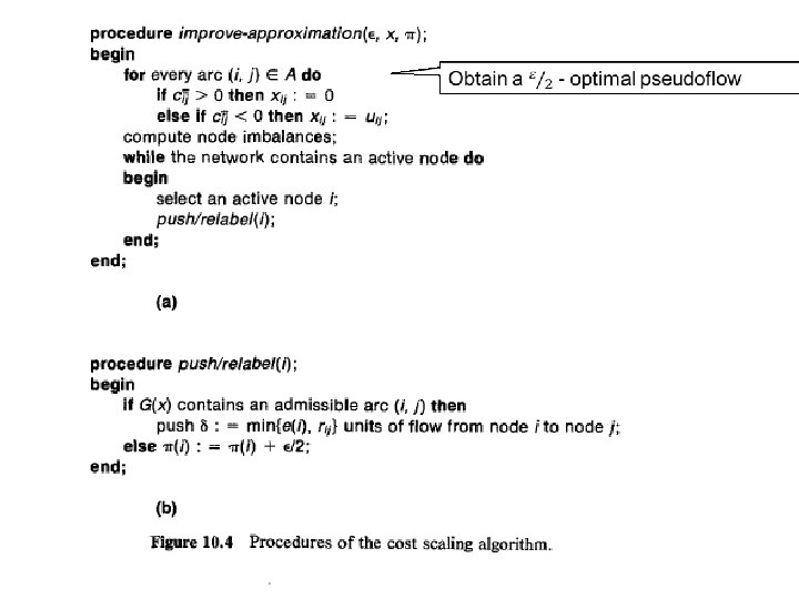
Algorithm Strategy

Preflow Push Recap

Distance Labels • Distance Labels Satisfy: • d(t) = 0, d(s) = n • d(v) ≤ d(w) + 1 if r(v, w) > 0 • d(v) is at most the distance from v to t in the residual network. • s must be disconnected from t …

Terms • Nodes with positive excess are called active. • Admissible arc in the residual graph: v w d(v) = d(w) + 1

The preflow push algorithm While there is an active node { pick an active node v and push/relabel(v) } Push/relabel(v) { If there is an admissible arc (v, w) then { push = min {e(v) , r(v, w)} flow from v to w } else { d(v) : = min{d(w) + 1 | r(v, w) > 0} (relabel) }

Running Time • The # of relabelings is (2 n-1)(n-2) < 2 n 2 • The # of saturating pushes is at most 2 nm • The # of nonsaturating pushes is at most 4 n 2 m – using potential Φ = Σv active d(v)

Back to Min Cost Flow…

Applying Preflow Push’s technique i j

Initialization -10 v w

Push/relabel until no active nodes exist

Correctness • Lemma 1: Let x be pseudo-flow, and x’ a feasible flow. Then, for every node v with excess in x, there exists a path P in G(x) ending at a node w with deficit, and its reversal is a path in G(x’). • Proof: Look at the difference x’-x, and observe the underlying graph (edges with negative difference are reversed).

Lemma 1: Proof Cont. • Proof: Look at the difference x’-x, and observe the underlying graph (edges with negative difference are reversed). 3 3 4 2 0 1 3 3 2 4 3 - 3 4 2 5 2

Lemma 1: Proof Cont. • Proof: Look at the difference x’-x, and observe the underlying graph (edges with negative difference are reversed). w v S • There must be a node with deficit reachable, otherwise x’ isn’t feasible

Correctness (cont) Corollary: There is an outgoing residual arc incident with every active vertex Corollary: So we can push/relabel as long as there is an active vertex

Correctness – Cont.

Correctness – Cont.

Correctness – Cont.

Correctness (cont)

Complexity • Lemma : a node is relabeled at most 3 n times.

Lemma 2 – Cont.

Lemma 2 – Cont.

Lemma 2 – Cont.

Complexity Analysis (Cont. ) • Lemma: The # of saturating pushes is at most O(nm). • Proof: same as in Preflow Push.

Complexity Analysis – non Saturating Pushes • Def: The admissible network is the graph of admissible edges. -2 4 2 2 -2 -1 -4

Complexity Analysis – non Saturating Pushes • Def: The admissible network is the graph of admissible edges. -2 -2 -1 -4

Complexity Analysis – non Saturating Pushes • Def: The admissible network is the graph of admissible edges. • Lemma: The admissible network is acyclic throughout the algorithm. • Proof: induction.

Complexity Analysis – non Saturating Pushes – Cont. • Lemma: The # of nonsaturating pushes is O(n 2 m). • Proof: Let g(i) be the # of nodes reachable from i in admissible network • Let Φ = Σi active g(i)

Complexity Analysis – non Saturating Pushes – Cont. • Φ = Σi active g(i) • By acyclicity, decreases (by at least one) by every nonsaturating push i j

Complexity Analysis – non Saturating Pushes – Cont. • Φ = Σi active g(i) • Initially g(i) = 1. • Increases by at most n by a saturating push : total increase O(n 2 m) • Increases by each relabeling by at most n (no incoming edges become admissible): total increase < O(n 3) • O(n 2 m) non saturating pushes

Cost Scaling Summary • Total complexity O(n 2 mlog(n. C)). • Can be improved using ideas used to improve preflow push

Double Scaling (If Time Permits)

Double Scaling Idea

Network Transformation b(i) i Cij, uij xij b(j) b(i) j i Cij, xij -uij 0, (i, j) b(j) j rij

Improve approximation Initialization N 1 N 2 +

Capacity Scaling - Scheme

Double Scaling - Correctness • Assuming algorithm ends, immediate, since we augment along admissible path. • (Residual path from excess to node to deficit node always exists – see cost scaling algorithm) • We relabel when indeed no outgoing admissible edges.

Double Scaling - Complexity • O(log U) phases. • In each phase, each augmentation clears a node from S( ) and doesn’t introduce a new one. so O(m) augmentations per phase.

Double Scaling Complexity – Cont. • In each augmentation, • We find a path of length at most 2 n (admissible network is acyclic and bipartite) • Need to account retreats.

Double Scaling Complexity – Cont. • In each retreat, we relabel. • Using above lemma, potential cannot grow more than O(l), where l is a length of path to a deficit node. • Since graph is bipartite, l = O(n). • So in all augmentations, O(n (m+n)) = O(mn) retreats. N 1 N 2

Double Scaling Complexity – Cont. • To sum up: • Implemented improve-approximation using capacity scaling • O(log U) phases. • O(m) augmentations per phase. • O(n) nodes in path • O(mn) node retreats in total. • Total complexity: O(log(n. C) log(U) mn)

Thank You