Microsoft Office Excel Topic 1 Excel Terms Selecting

Microsoft Office: Excel

Topic 1: Excel Terms & Selecting Cells

Objective: - Define terms used in Excel. - Identify ways to select cells in a workbook.

Excel Window Terms To Know: Spreadsheet- Document that is entirely made up of rows and columns. Used to list and analyze data. To add to the confusion in the world, people tend to use the word spreadsheet in two ways: �the entire Excel workbook file �an individual worksheet Workbook- Made up of several worksheets saved together. A workbook is the basic document for Excel. Its filename uses the extension xls, from Excel spreadsheet. A workbook usually contains several worksheets.

Excel Window Terms To Know: Worksheet- An individual page within Excel. One or more worksheets make a workbook. Think of them as pieces of paper that are stacked on top of each other to form the workbook. The maximum number of worksheets in a workbook depends on your computer's memory. A workbook does not have a maximum number of worksheets- it is limited only by the amount of memory your computer has to work with. . A worksheet, also called just a sheet or spreadsheet, can have up to 16, 384 columns and 1, 048, 576 rows with up to 32, 767 characters in a single cell. This is more than enough for most purposes!

Cell- An individual box on a worksheet. It is the intersection of a row and a column on a worksheet. Sheet Tabs- Allow you to move from one worksheet to another. Each worksheet has a tab at the bottom of the workbook window with the name of the worksheet on it.

Excel Window Terms To Know: Active Worksheet- The worksheet that you are currently working in. It has a white tab and its name is bold. Workspace- The area below the toolbars that holds your documents The default workbook is named Book 1. It contains one worksheet named Sheet 1, however you can add as many as you need with the “+” sign. You can change the names of each sheet to better identify what is found on each page.

The Worksheet & Formula Bar Name Box Row Header Column Row

Worksheet & Formula Bar Terms to Know: Columns- Lines on a worksheet going up and down. Columns are named with letters in the following pattern: A, B, C, …Z, AA, AB, AC, …AZ, BA, BB, BC, …BZ, up to XFD, which is the last possible column for a total of 16, 384 columns. Rows- Lines on a worksheet going side to side. Named with numbers from 1 to 1, 048, 576.

Worksheet & Formula Bar Terms to Know: Headings- The gray buttons at the top of columns and at the left end of rows Cell- The intersection of a column and a row Cell Reference - A combination of letters and numbers that names a cell. This is how we refer to a cell, using the letter of the cell's column followed by the number of the cell's row, like B 3 or AD 345.

Worksheet & Formula Bar Terms to Know: Name Box- This is where the cell reference is shown. It is found at the top left above the sheet and to the left of the formula bar. Formula Bar- This is where you type in the information that will be shown in a cell. It shows the contents of a selected cell, whether it is plain text, numbers, or a calculation formula.

Worksheet & Formula Bar Terms to Know: Formula- Will allow Excel to perform calculations for you. They look like an algebra equation, like =SUM(A 4: D 7) or =AVERAGE(C 3, F 5, H 10). Most formulas use cell references to get the values to calculate with. = (Equals Sign)- Used at the beginning of all formulas. A formula will not work in Excel without the = sign.

Worksheet & Formula Bar Terms to Know: Active Cell- Has a dark border around it. The row and column headers are either raised, like buttons, or are colored, depending on your version of Excel. This is the cell that you are currently typing in. You make a cell the active cell when you select it, by clicking it or by moving into it with keys. The TAB or the arrow keys are handy for moving from cell to cell.

Worksheet & Formula Bar Terms to Know: Range- A range represents a group of cells and is referred to by using the upper left and lower right cell references with a colon between them, like A 3: C 6 for the range illustrated below. Ranges are used in formulas

Worksheet & Formula Bar Terms to Know: Hidden contents: Information in a cell can be partially hidden if the cell next to it is filled with data. None of the cell data is lost. You just can't see it. The Formula bar shows all the text in the selected cell. If the cell to the right is empty, the contents of a cell will overlap into the next cell.

Pointer Shapes The mouse pointer has a number of shapes in Excel. The shape indicates what the effect will be of your mouse actions and keystrokes. As you move the pointer around, it may flicker from one shape to another.

Shape: Used To:

Shape: Used To:

Selecting A Range of Cells To select a range of cells that are touching : - Click & Drag, - Hold down Shift, click the first and last cell, and the ones in between will be selected or To select cells that are not touching: - Hold down CTRL and click cells to be selected

To Select a Range Using SHIFT: -Click B 3 -Hold Down SHIFT -Click B 14 All of the cells between B 3 and B 14 should be highlighted. This also works to select multiple rows or columns.

To Select Multiple Cells That Are Not Touching Using CTRL: -Click A 3 Then hold Down CTRL -Click C 5, D 3, E 5, F 3 All five of the cells you clicked on should be highlighted. This also works to select multiple Rows or Columns.

Selecting Rows and Columns When you hover a header, your pointer will become a solid back arrow. When you click the header (Letter or Number), the entire row or column will be selected. To select multiple columns and rows, continue to press down on the mouse button and drag. If you need to delete a row or column, R Click after you have selected them and choose “Delete”.

Selecting All Cells on a Worksheet If you need to select every cell on a page, click the triangle button that is found between Header A and Header 1. This is helpful if you want to change the style of the text or borders on the entire page.

Selecting Sheets To select worksheets, click the tabs at the bottom of the workbook window. The tab selected will have its name underlined and displayed in color. Why would you want to select sheets? �To rearrange their order �To copy sheet(s) to a new spreadsheet �To perform the same action on all the selected sheets at once.

Changing Tab Labels and Color The Tab Label at the bottom of each Worksheet can be renamed from “Sheet 1” to whatever you like within 30 Characters. The color of the tab can also be changed to make it easy to identify worksheets at a glance. More worksheets can also be added, up to a maximum of 255.

To Rename A Tab 1. 2. 3. Right Click on the Worksheet Tab Select “Rename” from the Menu Type in the new name directly on the Tab

To Change A Tab’s Color 1. 2. 3. Right Click on the Worksheet Tab Select “Tab Color” from the Menu Click on the color that you want the Tab to be. Click OK.

To Add A Worksheet 1. 2. Click the “+” sign next to the last tab displayed The new sheet appears to the Right of the tab you were in when you added a new tab. Since I was on “Sheet 2” when I clicked the +, “Sheet 4” was added to the right of it.

To Rearrange Worksheets Click and Hold Down on the Worksheet Tab. Your pointer will have a sheet of paper appear above it. 2. Drag the Worksheet to the Left or Right until it is in the order you want it. You will see a small triangle that will show you where the sheet will move. 3. Release the mouse button. 1.

To Delete A Worksheet 1. 2. 3. Right Click on the Worksheet Tab Select “Delete” from the Menu The Worksheet should disappear

Think It Through �Use the labels to identify the parts of the Excel Window. Cell Column Header Row Header Sheet Tab Scroll Bar Tabs Groups Row Formula Bar Name Box Add New Page Zoom Column

Think It Through �Use the labels to identify the parts of the Excel Window. Tabs TOP SECRET --No Peeking!— Groups Name Box ow ader Formula Bar Column Header Cell Row C o l u m n (Delete or drag this box over to check your answers) Sheet Tab Add New Page Scroll Bar

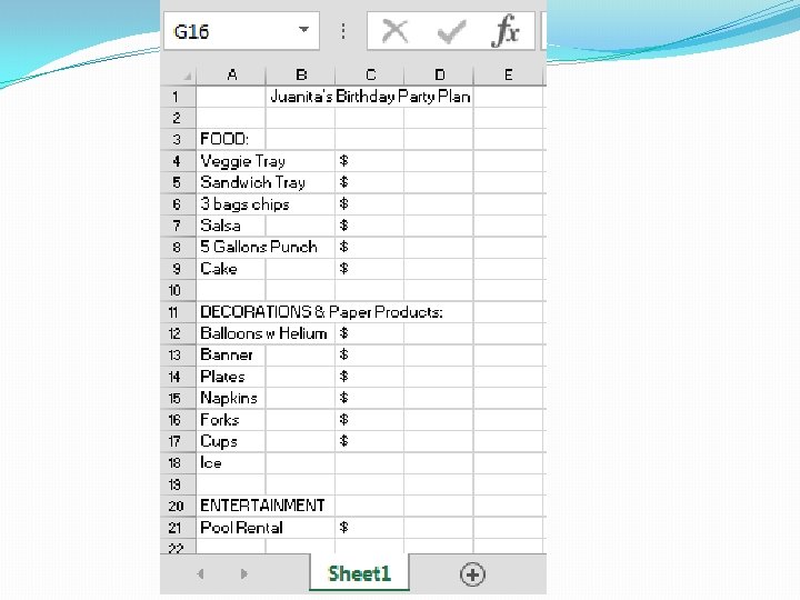
Think It Through On a new worksheet, practice entering data by listing the items you would need to plan for an upcoming birthday party with 20 guests. Use the internet to research the prices of these items and include the price in a separate column (Round price to the nearest dollar). Create your lists under the following headings: Food (Ex: Appetizers, Cake, Drinks) Decorations & Paper Products (Ex: Balloons, Banner, Plates, Cups, Forks, Napkins) Entertainment (DJ, Slide, Bounce House, or Venue Rental)

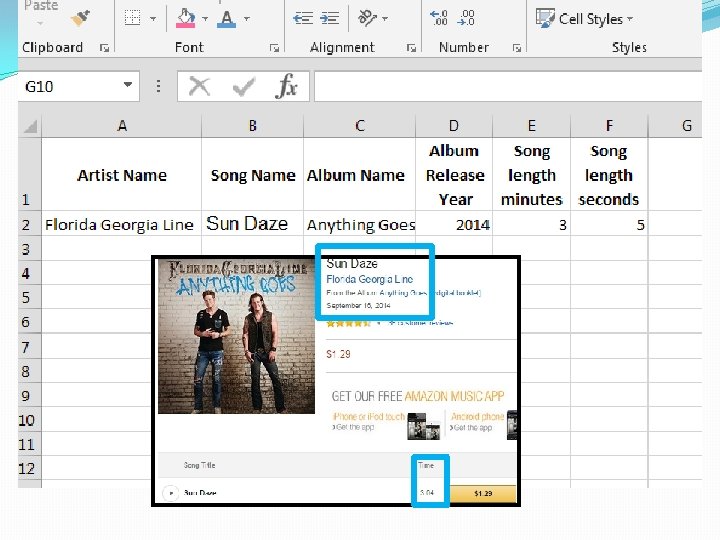
Think It Through In your Party Planning Workbook, create a new sheet and name it “Playlist”. Practice entering data by listing enough songs that you could play at your party for two hours (120 Minutes) without any song repeating. Include: Artist Name, Song Name, Album Name, Album Year Song length (minutes), Song Length (seconds) HINT: If you google the name of the song w MP 3 behind it, you can find a website that sells the song and it will show long the song is. Amazon is really good too.

“Excel”lent Art Creating art in Excel can be very time consuming- but if you can design and color a picture on graph paper, you could re-create it in Excel by adjusting columns and rows and using fill for color.

“Excel”lent Art Create your own art in Excel. Adjust the columns and rows so that they make perfect squares and use the bucket to fill the cells with color. The sad picture below was done using 15 pixel by 15 pixel columns and rows- you can see that there is very little detail, so you may need to make yours smaller than that and then zoom in. HINT: If you want your background to be a certain color (like the sky) do it first! Its Aggravating to go around the stuff You draw to fill in later.

Strive For Success �Time to check your understanding of Topic 1: Excel Terms & Selecting Cells �Our class will take a quiz on ____(Quiz Date)_______. �Use your Study Guide and Think It Through Activities to strive for success on the quiz!

Topic 2: Entering Data

Objective: - Enter & manipulate data in Excel manually and by using Auto. Fill Features.

Entering Data: Excel is not much different than Word or Power. Point when it comes to entering data (numbers or letters) however, there a few differences that you must get used to. Typing: To Type in a cell, simply select the cell by clicking in it. You can then type directly in the cell or type in the formula bar.

Formatting Text: You can Format text to be bold, underlined, aligned to a particular direction, and with different colors and fonts. When selecting text that you want to format, it is best to work from the formula bar. Highlight the text with your mouse and apply formatting changes from the “Font” group just as you would in Word.

Multiple Lines of Text: You can have Multiple Lines of text within one cell. When typing in a cell, hold down “Alt” and press “Enter” on the keyboard at the same time. This will move your curser down to a second line within the cell to create a second line. To better see the text in the formula bar, click the arrow at the end of it to expand your view.

Moving Text: You can Move text from one cell to another by using your mouse to drag it across the sheet. First, select a cell that you want to move, then hover your mouse on one of the four bold edges until you get a fourheaded arrow. As you start to drag the text, new cells will become highlighted. When the cell you want to move the data to is highlighted, release the mouse to drop the text.

Copying Text: You can Copy text from one cell to another by using your mouse. First, select a cell(s) that you want to copy, then R click on the cell and select “Copy”. The cell will become animated with green and white lines circling its border. Move to the cell you want to copy the data to and R click in the cell and select a Paste Option (one of several clipboards)

Repeat Text with Autofill: You can Repeat text from one cell to many cells by using your mouse. First, select a cell that you want to copy, then hover your mouse in the lower R corner where you see the green square. Your pointer will become a black “plus sign”. Drag the cell in any direction and it will fill or replace the surrounding cells with the same text that was in the original cell. +

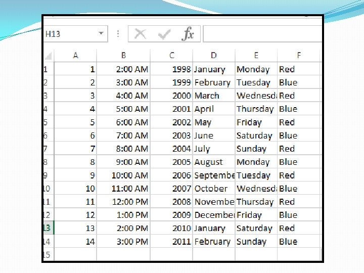
Entering Series of Data with Autofill: Excel has many built-in-series of data that you can Autofill, such as numbers, time, years, days of the week & months of the year. When you are creating lists and categories, this can be very timesaving. Begin by typing two sets of data that you would like Excel to continue, then select the cells with your mouse and hover in the lower R corner where you see the green square. Your pointer will become a black “plus sign”. Drag the cells in the direction you were working in (down or across) and it will continue your pattern in the following cells. See examples next slide

Merging Cells: You can combine two cells together using the “Merge” option in the “Alignment” group of the Home Tab. Merging two or more cells will combine them into one large cell. However, it will delete all cell contents except for the data that is found in the first (Upper Left) cell of the group you have selected. + If you want to change it back, select the cell and click “Unmerge”

Clearing and Deleting Cells: If you need to empty out a cell, you can either clear the contents or you can delete the cell. Clearing the Content will only delete the data in the cells, the cells will remain in place but will be empty. Select the cells you want to clear, R Click and choose “clear contents”. Deleting cell actually removes the cells and the remaining cells around the ones removed will shift into the space left by the deleted cells. Select the cells you want to delete, R Click and choose “delete”. See example next slide

Clearing vs Deleting Cells: Original Column D was cleared. Empty cells now remain in Column D was deleted. Columns E & F have now shifted Left one space to become Columns D & E

Think It Through In Cell A 1 - Type Ponchatoula. In Cell B 1 - Type Junior High School. Format it to be Arial, green, size 14 In Cell C 1 - Type 8 th Grade. Make a second line (Alt + Enter) and type Ms Lee’s Class below. In Cell D 1 and D 2 type the first two month of the year and use Auto. Fill to continue the series. Use the Name Box to navigate to cell CD 11177. Type Supernerd in this cell. Merge the months April and May together. Use the Name Box (XFD 1048576) or navigation keys (Ctrl + , Ctrl + ) to navigate to and type LAST CELL in the last cell of the worksheet. Add Worksheet 2 - Name the tab “Practice” Copy all of the text from Sheet 1 and copy/paste it onto the “Practice” Sheet (Sheet 2)

Strive For Success �Time to check your understanding of Topic 2: Entering Data �Our class will take a quiz on ____(Quiz Date)_______. �Use your Study Guide and Think It Through Activities to strive for success on the quiz!

Topic 3: Sorting & Formatting Cells

Objective: - Format Cell Appearance with Color, Fill and Borders - Sort Data

Arranging Data: Excel allows you to organize data. Both the order of data and the layout of the worksheet can be changed. This is most often done with sorting, adjusting columns, and adjusting rows.

Sorting can help rearrange your data so you can use it more efficiently. It helps you look at the same data in different ways at different times. Example: In a list of students at PJHS, I may want to look for a student by name, grade, homeroom, birthday, or phone number. Excel will allow me to change the list to do this.

Basic Sorting �Excel allows you to sort in regular alphabetic or numerical order and in reverse order with the buttons Sort A-Z and Sort Z -A �You can sort whole rows or sort just selected cells, based on the first column of the selection

�For a basic sort, select the column and choose A-Z or Z-A and the column of data will be arranged in the order you chose. �If the column you selected has another row of data touching it, Excel will ask you if you want to “Expand the selection”

�If you select “Expand the selection”, Excel will keep the data touching your column attached to the cell it is currently touching and sort them together. So when Audi moves to the top of the list, so will S 4 - the cell that was next to it. �If you choose “Continue with the current selection”, it will ONLY sort the column you selected and the column attached to it will remain as it is. So now it look like Audi makes the F 150. Expand Continue

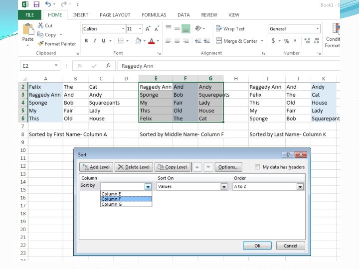
Custom Sorting �For a sorting when there are multiple columns of data near one another, a Custom Sort may be needed. Select the sections of data you want to work with and choose “Custom Sort”. A menu will open that allows you to select the column that you want the information sorted by. This feature is important when you have data in other columns that you do not want re-arranged.

Formatting Columns You can apply almost every kind of formatting to whole columns at once. Just select the column(s) and apply the formatting. This is handy when a whole column should have bold text, for example, or the same type Font. Column Width: The formatting that is unique to columns is Column Width. There are several methods that you can use to adjust the width of your columns. Each is most useful in certain circumstances, so you do need to be aware of them all.

Column Width: Dragging is a natural method of adjusting column width. But since you can't see the change until you release the mouse button, it may take you several attempts to get a satisfactory width. Move the pointer to the right edge of a column heading. When the pointer changes to the “Resize Column” (double headed arrow) shape, drag to the right until it reaches a width you like.

Column Width: Auto. Fit Selection You sometimes want a column to be wide enough for a particular cell's contents, but want other cells to wrap any longer lines in them. 1. Select the cell that you want to determine the column width 2. Home Tab>Cells Group> Format> Autofit Column Width The column is resized just wide enough to hold the text in the cell you selected.

Column B will became only as wide as the word “Old”

Column Width: Auto. Fit All Move your pointer to the right edge of the heading of a Column until it changes to the Resize Column shape. Doubleclick in the same spot (the right edge of the Column’s heading). The column width changes to be as wide as the longest text in any cell in the column. TIP: If you L click on the right edge of the heading of a Column, a popup tip appears showing the current width of the Column.

Column Width: Dialog Box Select a cell Choose Home Tab>Cells Group> Format> Column Width The Column Width dialog appears. Type a new width number and click OK

Formatting Cells and Borders You can change the color of cells, content, and the borders around the cells to make your spreadsheet look any way that you’d like. You must first select the cells that you want to format. Refer back to Slides 35 -38.

Change a cell’s fill or shading by going to the “bucket” on the Home toolbar or……

Go to Home Tab>Cells Group> Format Cells to select shades and patterns

If you want a pattern as your cell’s fill, choose the drop down menu below Pattern Color. FYI: The color palate on LEFT is for the cell background. The color palate on RIGHT is the color of the pattern.

Change what part of the cell’s border is seen by going to the border button on the toolbar or……

Go to Home Tab> Cells Group> Format Cells to select border style and color

Think It Through Practice Activity After we practice, you should be able to: 1. Adjust column width and row height. 2. Sort lists several ways. 3. Insert columns and be able to cut/paste columns or drag to re-arrange them. 4. Insert a formula to calculate a SUM 5. Format the table using borders and background fill. Format text color/ font.

Think It Through Family Names, Ages, and Gender 1. Create a Worksheet that lists at least 5 people (Real or Made. Up). Include 5 Columns for their First Name, Middle Name, Last Name, Age, and Gender. 2. Format the Chart: Use Yellow Fill for Headings. Fill each person’s row with Blue or Pink Fill depending on Gender. Make it have a Black Outside Border and Red Inside Borders. Make Columns 15 Wide and Rows 20 Tall. 3. Sort the Chart into ABC order based on Last Name. 4. Copy the Chart and paste the copy below the first. 5. Re-Sort the Chart based on Age. 6. Copy the Chart and paste in the copy below the second. 7. Re-Sort the Chart based on Gender. 8. Insert a formula to add everyone’s age in the last chart only.

Think It Through Play-List Assignment Directions: Today you will be researching some of your favorite songs/artists/bands. The plan is to create a play-list of 12 songs that you would like to listen to on your MP 3 player. You can use any website (that is not blocked) to find the information required. You will probably have to research the date of the album or song’s release. You are ranking the song from 1 -5 with 1 being worst and 5 being best.

Artist Last Name Lee Morgan Artist First Name ter n E Alt + 2 nd Line et To g Album Title Album Release Date Track Length Your Rank (1 -5 Star) Juanita PJHS scares the living bleep out of me 8 th Grade Misery is only short term, but Ms Lee is forever. 2008 2: 23 1 Beastie Boys The New Style License to Ill 1986 4: 36 4 Craig Almost Home I Love It 2003 4: 49 5 3 OH!3 Holler Til You Pass Out 3 OH!3 4: 01 3 Song Title 2007 Directions: Find the worksheet that you used to collect the Play-List songs. Type the 13 Rows of Information into a new Excel Spreadsheet. Save it to Your Documents as “Last. Name. Playlist”. See next slide for Formatting Requirements.

Formatting Requirements 1. 2. 3. 4. 5. 6. 7. 8. 9. 10. Fill the cells using a three color combination. One color should be used on the headings. The other two colors should be used on alternating lines below the header. See example on previous slide. Text may be any color that is easy to read. Please leave the font as Ariel and make it size 12. Use “Auto. Fit” to format the Artists Last Name. Format the rest of the columns so that they are the same widths. Make all rows a height of 17. Use “Auto Sum” to add up all 12 track lengths below the last time. Use “Average” to find the average rank of all 12 songs below the last rank. Choose a color for the outside border and inside borders. They can not be the same. Please use thickest line style. Please use a solid line- not dashed. Re-Name the tab of the worksheet you are working on “Playlist” Make the tab color the same as your header Delete worksheets 2 and 3 Save as “Last Name Playlist” to the assignment drive

Strive For Success �Time to check your understanding of Topic 3: Formatting & Sorting Cells �Our class will take a quiz on ____(Quiz Date)_______. �Use your Study Guide and Think It Through Activities to strive for success on the quiz!

Topic 4: Excel Chart Wizard

Objective: - Create Charts in Excel using the Chart Wizard

Vocabulary: Chart wizard- The guide or process to help users create a chart in Excel Chart – A graphical representation of data in a worksheet. Chart types – Column, Bar, Line, Pie, 2 D/3 D Chart sheet – A chart that occupies its own worksheet. Embedded chart – A chart placed as an object within a worksheet.

Vocabulary: Categories- The information in a worksheet row. You will have multiple categories if more than one row is selected. (The colors of M&M’s are the categories) Data series –The information in a worksheet column. If you select more than one column, then you have multiple data series. (This chart has only one series. If we added the data from another bag in column C, there would be multiple series)

Vocabulary: Title- The title at the top of a chart describing the chart Legend – A key that identifies each of the data series in the chart.

Vocabulary: X-axis – The horizontal (side to side) scale on a chart on which categories are plotted. Y-axis – The vertical scale (Up and down) of a chart on which the value of each category is plotted. Plot area – The area defined by the x and y axes. Slice- A fractional part of pie chart Bars/Columns/Slices- Should be different colors or patterns in your chart

Charts �The Charts in Excel is another of its useful features. You can easily create charts of various kinds using spreadsheet data. The wizard leads you step by step to turn numbers into cool and colorful charts.

Insert Tab: Charts The chart wizard helps you to easily create line, bar, and pie charts. Step 1: Select a group of data by clicking and dragging over it with your mouse.

Step 2: Choose the Chart Type that you want to work with. There are many to choose from including Bar, Line, Column and Pie Graphs.

Step 3: The Graph will appear on your worksheet. You can edit the title on the graph by double clicking the text box

Step 4: Adjust colors the graph by double clicking the color of the chart you wish to change. Select new colors from the task pane that opens.

You can also adjust the color of the Background (Fill) of the chart and the Border (Line) surrounding it.

When you click the chart, three menu items will appear on the right of the chart. Chart Elements, Styles and Filters.

Chart Elements: Here you can format chart Titles, Labels, Axis and Legend.

Chart Styles: Here you can format the style and colors used in your chart

Chart Filters: Here you can turn data “on and off” to remove it from view in a chart.

Chart Tools: Design Tab Once you create a chart, the Chart Tools Tab will appear. It has two tabs: Design and Format.

Bar Graph Activity Pick an item from this slide or the next to work with. Count how many there are of each color and put the information on a blank Workbook. Use the Chart group of the Insert Tab to create a Graph. Use the M&M Graph sample to help you.

Bar Graph Activity Pick an item from this slide or the previous to work with. Count how many there are of each color and put the information in a blank Workbook. Use the Chart group of the Insert Tab to create a Graph. Use the M&M Graph sample to help you.

Line Graph Activity We will count your heart rate while: Sitting at rest Taking a quiz Walking down the hall Walking up the stairs Running up the stairs *The easiest way to count your heart rate is to find your pulse on your neck for 10 seconds and then multiply by 6.

Sample

Strive For Success �Time to check your understanding of Topic 4: Excel Chart Wizard �Our class will take a quiz on ____(Quiz Date)_______. �Use your Study Guide and Think It Through Activities to strive for success on the quiz!

Topic 5: Using Formulas

Objective: - Use Formulas and Auto. Fill in Excel to organize data.

Addition =SUM(B 1: B 3) =SUM(B 1, B 2, B 3) =B 1+B 2+B 3 To add, use the formula =SUM or the + sign. Put the range (two cell references with a colon between them) of numbers you wish to be added in parentheses. If you only want some of the numbers added together, put a comma between the cell references. You can include more than two and they do not have to come from the same row.

Addition with Formula and Range =SUM(B 1: B 3) Put the range (two cell references with a colon between them) of numbers you wish to be added in parentheses. In this example, we added all of the colors. B 2 : B 7

Addition with Formula and Comma =SUM(B 1, B 2, B 3) If you only want some of the numbers added together, put a comma between the cell references. In this example, we added only Orange and Green. B 2 , B 5

Addition with Cell Reference and + Sign =B 1+B 2+B 3 If you only want some of the numbers added together, you can also type Cell References with + Sign between them. In this example, we added only Yellow and Blue. B 3 , B 7

Subtraction =B 3 -B 2 -B 1 To subtract, use the subtraction sign (found to the Right of the number zero) between two or more cell references. You can include more than two and they do not have to come from the same row. Unlike addition, there is not a subtraction formula that can be used.

Subtraction =B 3 -B 2 -B 1 In this example, we subtracted Yellow From Red. B 4 - B 3

Multiplication =PRODUCT (B 3: B 5) =PRODUCT(B 5, B 6) =B 3*B 4*B 5*B 6 To multiply, use the formula =PRODUCT or the * sign. Put a comma between the cell references you wish to multiply in parentheses. If you want several numbers to be multiplied, put the range (two cell references with a colon between them) of numbers in parentheses. Numbers do not have to come from the same row.

Multiplication with Formula and Range =PRODUCT (B 3: B 5) In this example, we multiplied Yellow times Red times Green. B 3 : B 5

Multiplication with Formula and Comma =PRODUCT(B 5, B 6) In this example, we multiplied only Green and Blue B 5, B 6

Multiplication with Cell Reference and * Sign =B 3*B 4*B 5*B 6 In this example, we multiplied Yellow, Red, Green and Blue B 3*B 4*B 5*B 6

Division = B 5/B 3 = B 9/B 5/B 3 To divide, use the forward slash sign (found to the Left of the Right shift key) between two or more cell references. You can include more than two and they do not have to come from the same row. Unlike multiplication, there is not a division formula that can be used.

Division = B 5/B 3 = B 9/B 5/B 3 Difference

Counting =COUNT(A 2: A 5, B 4: B 6) If you have many cells of data and you’d like to know how many there are, Excel will count the cells for you. Excel will ONLY count cells that have NUMBERS in them. In this example, 7 cells are included in the formula but only three have numbers in them, so the count is three.

Numbering =ROW(A 1) If you are making a list and you would like the list numbered, Excel will do it for you. In the box that you would like the number 1 to begin, insert the formula =ROW(A 1). In the lower R corner, you will be able to drag down to the last cell you want numbered. When you release, the numbers will appear. If you wish to start at a number other than 1 (such as if you needed to skip a few cells between lists), enter that number in the cell reference instead of 1. Ex- to begin at 7 enter =ROW (A 7)

A 2: A 7 used the formula =ROW(A 1) because it began counting at the number 1 A 9: A 13 used the formula =ROW(A 7) because it began counting at the number 7

Averaging =AVERAGE(B 2: B 7, B 10: B 15) To average numbers (To add up a total and divide by the how many numbers there are), use the formula =AVERAGE(B 2: B 7) with the cell reference of the range of numbers needed. If your numbers are found in more than one place, include multiple ranges with a comma between them =AVERAGE(B 2: B 7, B 10: B 15)

Averaging = AVERAGE(B 2: B 7)

Number Formats The following are formats can be applied to numbers in cells. This is found in the Numbers Group of the Home Tab. Currency: formats the number as money, like $1. 00 if your system is set to use dollars. Excel comes in different languages, and will use the appropriate local currency. Percent: formats the number as a percentage, like 100%.

Number Formulas Comma: formats the number to show 2 decimal places to the right of the decimal and uses commas to separate every 3 digits to the left of the decimal. Non -English versions of Excel may show a different button, . (Why doesn't the whole world do things the way I do? !) Increase/Decrease Decimals: changes the number of places showing to the right of the decimal. The number is rounded when decreasing decimals. When increasing decimals, the original digits are shown, rounded to the number of decimal places you have chosen.

Practice Activities When we finish the practice activity, you should be able to use Formulas to Add, Subtract, Divide, Find Averages and Count in Excel. Add: United States Facts Subtract: Bank Account Registry Divide: Density Calculator Find Average, Count: Grade Book (These files are found in the file: “Practice Activities For Excel” )

Addition: United States Facts

Subtraction: Bank Account Registry

Division: Density Calculator

Find Average, Count: Grade Book

Think It Through Fitness/ Health Assignment Use Excel to create tables that will help you log and calculate your: �Daily Food Log (Use addition formulas to calculate Caloric Intake) �Daily Exercise Log (Use addition formulas to calculate Caloric Expenditures. ) �Caloric Surplus/ Deficit (Use subtraction to compare your Exercise Log with your Food Log to determine if you have a caloric deficit or surplus) �Body Mass Index (Compares Height to Weight) Maximum Heart Rate (The highest heart rate you can safely reach for your age)

Daily Food Log Track all the foods you eat, research how many calories are in a serving, chart them and use addition formulas to calculate your Caloric Intake (Total sum of calories for the day) Use: http: //calorielookup. com/

Daily Exercise Log Track your daily exercise activities. Research how many calories are burned in a session, chart them, and use addition formulas to calculate your Caloric Expenditures. Use: http: //www. prohealth. com/weightloss/tools/ex ercise/calculator 1_2. cfm

Caloric Surplus/ Deficit Use subtraction to compare your Exercise Log to your Food Log. Determine if you had a caloric deficit or surplus for each day. Deficit- Means you burned more calories than you took in (weight loss) Surplus- Means that you consumed more calories than you burned. (weight gain)

Body Mass Index Use this formula as a guideline to build a calculator that will determine you (or anyone's) BMI based on Height and Weight: BMI = [ Weight in Pounds / ( Height in inches x Height in inches ) ] x 703 Ex: Ms Lee’s is: [170/ (702 )] x 703 =24

Maximum Heart Rate Use this formula as a guideline to build a calculator that will determine you (or anyone's) MHR based on Age: MHR= [211 - (64% x Age) ] Ex- Ms Lee’s is : [211 - (. 64 x 36)] = 188

Strive For Success �Time to check your understanding of Topic 5: Using Formulas �Our class will take a quiz on ____(Quiz Date)_______. �Use your Study Guide and Think It Through Activities to strive for success on the quiz!

Topic 6: Extra Tricks

Format the Background with an image Find a Picture or Map on Google Image Search that you would like to use as a background image. It must be at least 800 x 800 in size. Save it to your “My Documents”. > Uncheck “Gridlines”) HINT: You may need to past the picture in a PPT slide and save the slide as a JPEG so it does not tile in the workbook.

Format the Background with an image Apply that picture as the background of a new Excel worksheet. (Page Layout Tab> Background> Browse to Select File) While in Page Layout, uncheck “View Gridlines” to make the gridlines invisible. Options

Add Comments to Label The Picture Now that your background is an image, you can add comments to label the parts of the picture. The comments will not appear until someone hovers over the red triangle with their mouse. Options R Click in a cell and choose “Insert Comment” Type a description of whatever part is represented in that spot on the picture. Options

The comments will not appear until a user hovers over the red triangle with their mouse.

References This file was created/edited the summer of 2015 for the Tangipahoa Parish School System to teach 7 th Grade Computer Literacy for the 2015 -2016 School Year. Information found within this presentation was collected from Microsoft Digital Literacy & Support websites or created by the author. Digital Literacy: https: //www. microsoft. com/about/corporatecitizenship/giving/programs/up/digi talliteracy/default. mspx Support: http: //support. microsoft. com/ Images included in the presentation were found using a Google Image Search, specifically images tagged “Labeled for Reuse”. Screen Captures were taken from the TANGI Windows 7 Operating System or a program within the Microsoft Office 2013 Suite. Only Tangipahoa Parish School System teachers may copy, edit and reproduce this file and others within the series. Please email any questions regarding use of this and other files in the series. JLEE