Microsoft Excel Creating a Worksheet and an Embedded

Microsoft Excel Creating a Worksheet and an Embedded Chart
Excel Important Vocab Active cell Column Command group Command tabs Name box Quick Access Toolbar Ribbon Row Screen. Tips Workbook Worksheet Screen Tips Workbook Worksheet
Microsoft 2016 The foundation of Excel and locations where you do your work are Cells Rows Columns Worksheets are part of the workbook. Each tab is divided into task-specific command groups with commands and options that relate to the group name.
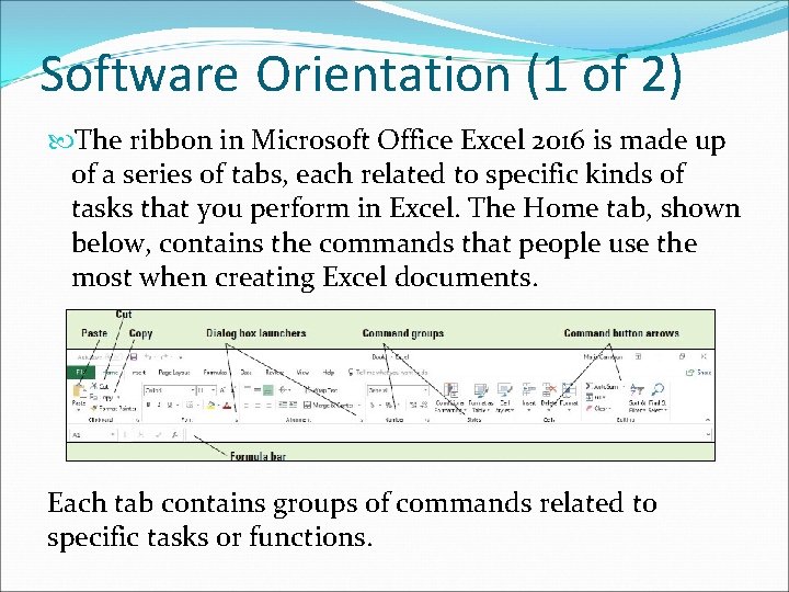
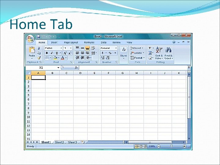
Software Orientation (1 of 2) The ribbon in Microsoft Office Excel 2016 is made up of a series of tabs, each related to specific kinds of tasks that you perform in Excel. The Home tab, shown below, contains the commands that people use the most when creating Excel documents. Each tab contains groups of commands related to specific tasks or functions.
Software Orientation (2 of 2) Commands that have an arrow associated with them (see Auto. Sum and Find & Select on the previous slide) have other options available for the task. The Dialog Box Launchers in groups display additional commands not shown on the ribbon. In the figure on the previous slide, the Clipboard, Font, Alignment, and Number groups have associated dialog boxes or task panes, whereas Styles, Cells, and Editing do not.
What is Excel? A powerful spreadsheet program that lets users to organize data, complete calculations, make decisions, graph data.
The 4 major parts of Excel Workbooks and Worksheets Charts Tables Web support
When Excel Starts… It creates a new blank workbook called Book 1
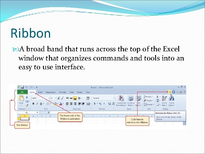
Ribbon A broad band that runs across the top of the Excel window that organizes commands and tools into an easy to use interface.
Workbook Is like a notebook. It is made up of column and rows Data is put in the cells of the workbook.
Worksheet Spreadsheets inside the workbook. Excel opens a new workbook with 3 sheets. You can additional worksheets as long as your computer has enough memory to accommodate them.
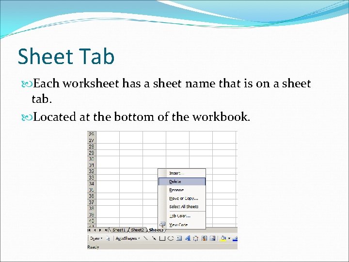
Sheet Tab Each worksheet has a sheet name that is on a sheet tab. Located at the bottom of the workbook.
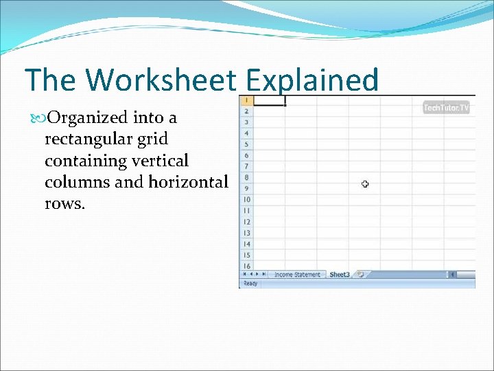
The Worksheet Explained Organized into a rectangular grid containing vertical columns and horizontal rows.
Cells in the Worksheet Active Cell A cell that is highlighted or outlined by a bold rectangle. This is also called the current cell or highlighted cell. A box on the worksheet grid identified by the intersection of a column and a row.

Command group Task-specific groups divided among the command tabs appropriate to the work a user currently performs.
What is a worksheet? A worksheet is a grid composed of rows, columns, and cells. Each worksheet column starts at the top of the worksheet and goes to the bottom of the worksheet and is identified by a letter. Each row starts at the left edge of the worksheet and continues to the right edge and is identified by a number. Each box, or cell, on the grid is identified by the intersection of a column and row.
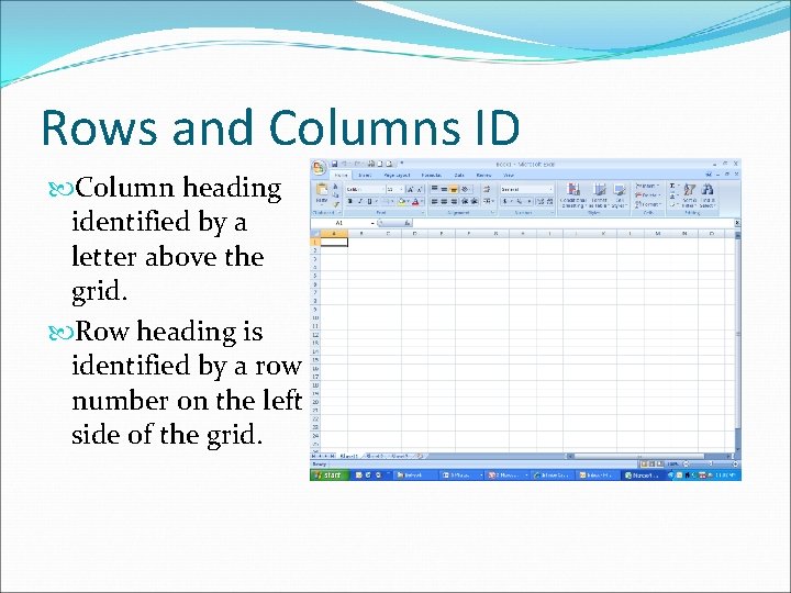
Rows and Columns ID Column heading identified by a letter above the grid. Row heading is identified by a row number on the left side of the grid.
A Workbook Spreadsheet file It can be compared to a physical book with many pages. When you open a blank workbook, the temporary filename (Book 1) and the program name (Excel) appear in the title bar at the top of the screen. Book 1 (or Book 2, Book 3, and so on) is a temporary title for your workbook until you save the workbook with a name of your choice.
A new Workbook The new workbook contains one worksheet (Sheet 1) by default. The sheet tabs are located just above the Status bar and are identified as Sheet 1, Sheet 2, and Sheet 3. (think of these as pages. ) Rename worksheets to identify their content. Add worksheets with the New sheet (+) button as needed.
What is a Cell? The intersection of each column and row A cell is a basic unit of a worksheet in which you enter data. Each worksheet has 16, 384 columns, 1, 048, 576 rows for a total of 17, 179, 869, 180 cells.
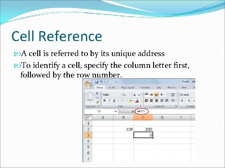
Cell Reference A cell is referred to by its unique address To identify a cell, specify the column letter first, followed by the row number.
Active Cell The one cell into which you can enter data. Active cell identified in 3 ways: A heavy border surrounds the cell Cell reference shows above column A in the Name box. The column heading and row heading are highlighted.
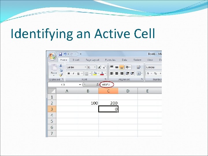
Identifying an Active Cell
Gridlines The horizontal and vertical lines on the worksheet itself. Gridlines make it easier to see and ID each cell in the worksheet. They can be turned off, but best to leave them on.
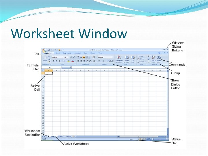
Worksheet Window
Worksheet Window You view the portion of the worksheet displayed on the screen through a worksheet window. Use the scroll bars, scroll arrows, and scroll boxes to move the worksheet around.
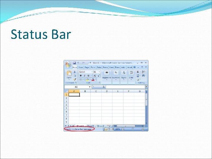
Status Bar
Status Bar Presents info about: the worksheet, the function of the button the mouse pointer is pointing to or the mode of Excel.
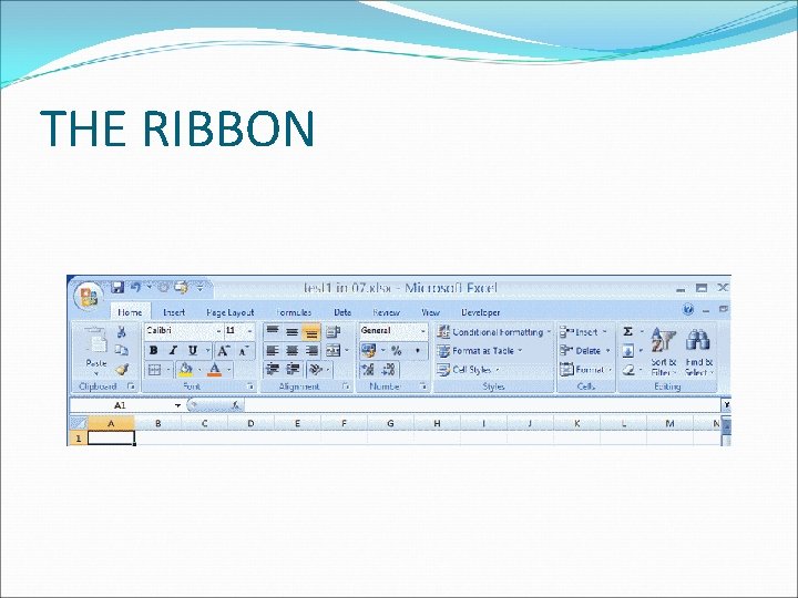
THE RIBBON
The Ribbon The control center in Excel Provides easy, central access to the tasks you perform while creating a worksheet. The ribbon has: Tabs, groups, and commands. Each tab surrounds a collection of groups Each group contains related commands.
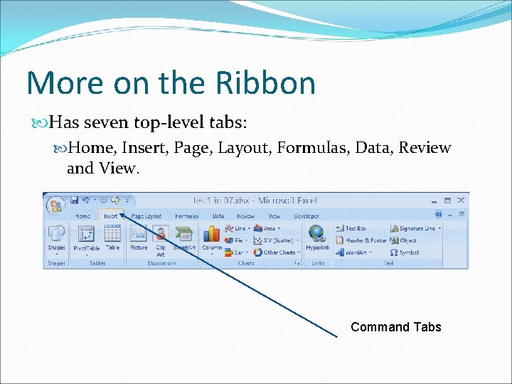
More on the Ribbon Has seven top-level tabs: Home, Insert, Page, Layout, Formulas, Data, Review and View. Command Tabs
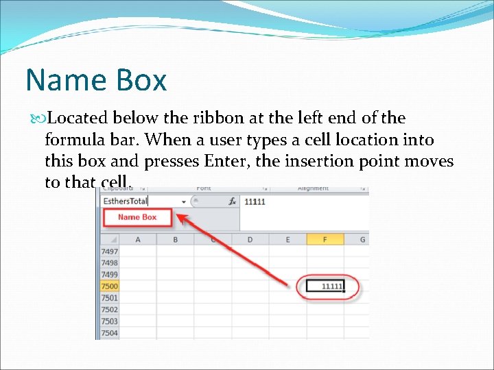
Name Box Located below the ribbon at the left end of the formula bar. When a user types a cell location into this box and presses Enter, the insertion point moves to that cell.
Home Tab
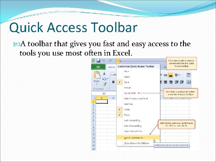
Quick Access Toolbar A toolbar that gives you fast and easy access to the tools you use most often in Excel.
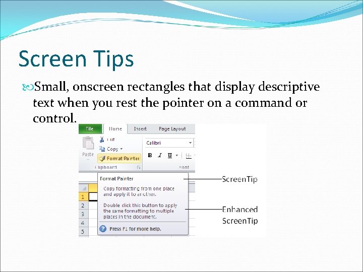
Screen Tips Small, onscreen rectangles that display descriptive text when you rest the pointer on a command or control.
Home Tab is. . Called the Primary tab Contains groups with the more frequently used commands. The active tab is the tab currently displayed.
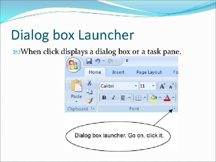
Dialog box Launcher When click displays a dialog box or a task pane.
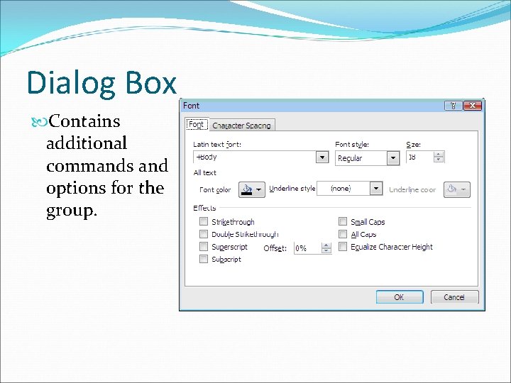
Dialog Box Contains additional commands and options for the group.
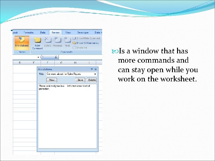
Task Pane Is a window that has more commands and can stay open while you work on the worksheet.
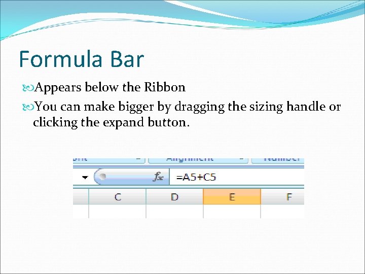
Formula Bar Appears below the Ribbon You can make bigger by dragging the sizing handle or clicking the expand button.
Splitting the Window When a worksheet contains a lot of data, you can see only a small portion of the worksheet in Excel’s Normal and page Layout views. The Split command enables to view the worksheet in two panes or four quadrants. The Split command lets you use the scroll bars on the right and at the bottom of the window to display different sections of the worksheet at the same time so you can compare or contrast data or see what effect a change in one part of the worksheet might have on a distant part of the worksheet.
Working with an Existing Workbook Many workbooks require frequent updating because existing data has changed or new data must be added. Workers frequently open an existing workbook, update information, and then save the workbook to be revised later. Filenames should reflect the type of data contained in the file and be descriptive so you can locate and retrieve files quickly. Filenames can be up to 255 characters long, including the filename extension. Most people use short descriptive filenames that clearly identify the content of the workbook.
Selecting a Cell To enter data into a cell, you first must select it. Easiest way to select a cell (make it active) is to use the mouse and click. Use the arrow keys to move around the spreadsheet.
Entering Text In Excel, any set of characters containing a letter, hyphen (as in a phone number) or space is considered text. Text is used to: Place worksheet titles, column titles, and row titles on the worksheet.
Alignment of Text Excel left-aligns text in a cell. Left-aligned means the cell entry is positioned at the far left in the cell. When text is longer than the width of a column, Excel shows the overflow characters in adjacent cells to the right as long as these adjacent cells contain no data.
Functions/Formulas AUTOSUM--a function used to add a column or row of numbers. AVERAGE—function used to add a series of numbers and then divide by the number in that series. MAX—function used to determine or identify the largest number in a group of selected number. MIN—function to identify the smallest number. Function—a built-in formula.
Navigating the Worksheet An Excel worksheet can contain more than one million rows and more than sixteen thousand columns. There are several ways to navigate through worksheets that contain numerous rows and columns: • Arrow keys • Scroll bars • The mouse
Navigating Data with the Go To Command The workbook used in these exercises is neither long nor particularly complicated. When dealing with much larger databases, or longer sets of workbooks, you might wish you had some easier means to get around the data than just scrolling. The Name Box indicates the current cell you are in as well as gives you the opportunity to name the cell or a range. The Go To command can take you to particular points in a worksheet, including cells and cell ranges that you name yourself.
Step by Step: Navigate Data with the Go To Command

Correcting Mistakes While Typing If you type the wrong letter, and see it before you hit ENTER, use the BACKSPACE key to delete characters.
Editing a Cell’s Contents Changes can be made quickly and easily in electronic records. To edit information in a worksheet, make changes directly in the cell or edit the contents of a cell in the formula bar. When you enter data in a cell, the text or numbers appear in the cell and in the formula bar. Before changes can be made, you must select the information that is to be changed. Selecting text means that you highlight the text to be changed. • You can select a single cell or a portion of the cell’s text in the formula bar. • You can also double-click in a cell to position the insertion point for editing.
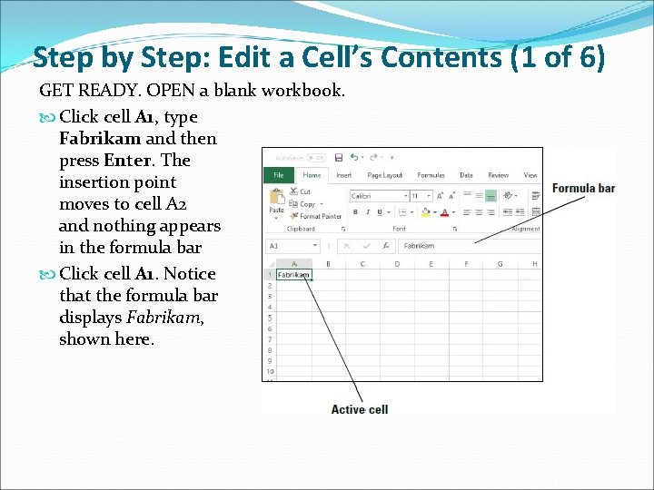
Step by Step: Edit a Cell’s Contents (1 of 6) GET READY. OPEN a blank workbook. Click cell A 1, type Fabrikam and then press Enter. The insertion point moves to cell A 2 and nothing appears in the formula bar Click cell A 1. Notice that the formula bar displays Fabrikam, shown here.
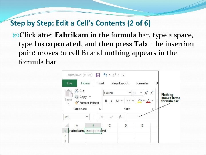
Step by Step: Edit a Cell’s Contents (2 of 6) Click after Fabrikam in the formula bar, type a space, type Incorporated, and then press Tab. The insertion point moves to cell B 1 and nothing appears in the formula bar
Step by Step: Edit a Cell’s Contents (3 of 6) 4. Click cell A 1 and in the formula bar, double-click on Incorporated to select it. Type Inc. and then press Enter. 5. Type Sales and then press Enter. 6. Click cell A 2 and then click after Sales in the formula bar. 7. Press Home. The insertion point moves to the beginning of the formula bar. 8. Type Monthly and then press the spacebar. Press Enter. 9. In cell A 3, type January and then press Enter.
Step by Step: Edit a Cell’s Contents (4 of 6) 10. Click cell A 3, type February, and then press Enter. Cell A 3’s original text is gone and February replaces January. 11. Click cell A 3 and then press Delete. The entry in cell A 3 is removed. 12. Above row 1 and to the left of column A, click the Select All button. All cells on the worksheet are selected. 13. Press Delete. All entries are removed. PAUSE. CLOSE the workbook without saving and LEAVE Excel open for the next exercise.
Step by Step: Edit a Cell’s Contents (5 of 6) When you are in Edit mode: • The insertion point appears as a vertical bar and most commands are inactive. • You can move the insertion point by using the left and right arrow keys. • The Edit indicator appears at the left end of the Status bar. Use the Home key on your keyboard to move the insertion point to the beginning of the cell, and use the End key to move the insertion point to the end of the cell. You can add new characters at the location of the insertion point.
Step by Step: Edit a Cell’s Contents (6 of 6) To select multiple characters while in Edit mode, press Shift while you press the arrow keys. You also can click and drag the mouse pointer over the characters that you want to select. There are several ways to modify the values or text you enter into a cell: • Erase the cell’s contents. • Replace the cell’s contents with something else. • Edit the cell’s contents.

Level 2 --Packet Formulas, Functions, Formatting and Web Queries
Using Data Types to Populate a Worksheet You can enter three types of data into Excel: text, numbers, and formulas. Text entries contain alphabetic characters and any other characters that do not have a purely numeric value. The strength of Excel is its capability to calculate and analyze numbers based on the numeric values you enter. Of course, if you enter the wrong numbers, you get the wrong calculations. For that reason, accurate data entry is crucial.
Entering Dates are often used in worksheets to track data over a specified period of time. Dates can be used as row and column headings. Dates are serial numbers. They are sequential and can be added, subtracted, and used in calculations. Dates can also be used in formulas and in developing graphs and charts. The way a date is displayed in a worksheet cell depends on the format in which you type the characters. In Excel 2016, the default date format uses four digits for the year and the date is right-justified.
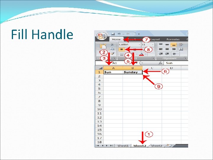
Filling a Series with Auto Fill Excel provides Auto Fill options that automatically fill cells with data and/or formatting. To populate a new cell with data that exists in an adjacent cell, use the Auto Fill feature either through the command or the fill handle. The fill handle is a small green square in the lowerright corner of a selected cell or range of cells. A range is a group of adjacent cells that you select to perform operations on all of the selected cells. When you refer to a range of cells, the first cell and last cell are separated by a colon (for example, C 4: H 4).
Filling a Series with Flash Fill allows you to quickly fill a column of data using an example that is based on existing data in adjacent columns. You can almost instantly create columns for first and last names if the full name appears in another column. After you enter the initial item (such as the first name) in a column and start to type the second item in that column, Excel displays a preview of entries formatted the same way in the rest of the column. If the presented preview of the data is what you want, just press Enter to fill the column with the entries.
Cutting, Copying, and Pasting Data Excel’s Cut, Copy, and Paste commands are used to copy or move entire cells with their contents, formats, and formulas. You can copy specific contents or attributes from the cells. You can copy the value from the original cell but retain the formatting of the destination cell. You can perform cut, copy, and paste functions using: • The mouse • Ribbon commands • Shortcut commands, such as Ctrl+C (copy), Ctrl+X (cut), and Ctrl+V (paste) • The Office Clipboard pane
Copying a Data Series with the Mouse By default, drag-and-drop editing is turned on so that you can use the mouse to copy (duplicate) or move cells. Select the cell or range of cells you want to copy and hold down Ctrl while you point to the border of the selection. When the pointer becomes a copy pointer (arrow with a plus), you can drag the cell or range of cells to the new location. As you drag, a scrolling Screen. Tip identifies where the selection will be copied if you release the mouse button.
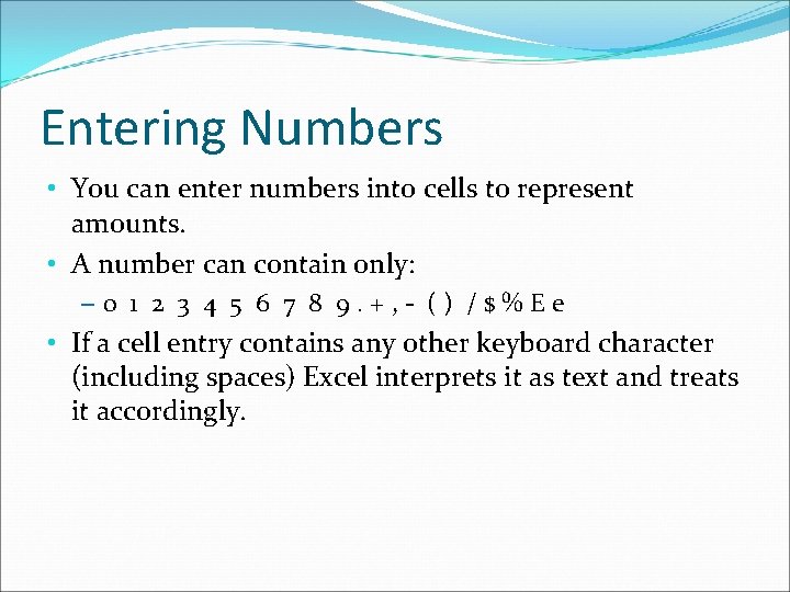
Entering Numbers • You can enter numbers into cells to represent amounts. • A number can contain only: – 0 1 2 3 4 5 6 7 8 9. + , - ( ) / $ % E e • If a cell entry contains any other keyboard character (including spaces) Excel interprets it as text and treats it accordingly.
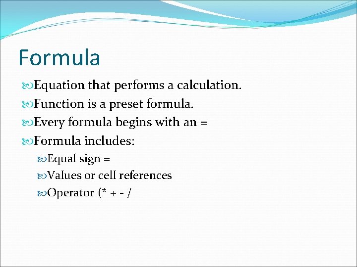
Formula Equation that performs a calculation. Function is a preset formula. Every formula begins with an = Formula includes: Equal sign = Values or cell references Operator (* + - /
Automatic Recalculation Every time you enter a value into a cell in the worksheet, Excel automatically recalculates all formulas.
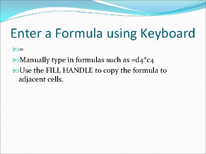
Enter a Formula using Keyboard = Manually type in formulas such as =d 4*c 4 Use the FILL HANDLE to copy the formula to adjacent cells.
Fill Handle
Point Mode An alternative to entering the formulas in cells Use the mouse to point and select cells for use in a formula. Even with Point Mode you must type the = and the operator (* + -, etc. )
When should I use Point Mode to Enter Formulas? Using Point mode to enter formulas often is faster and more accurate than using the keyboard.
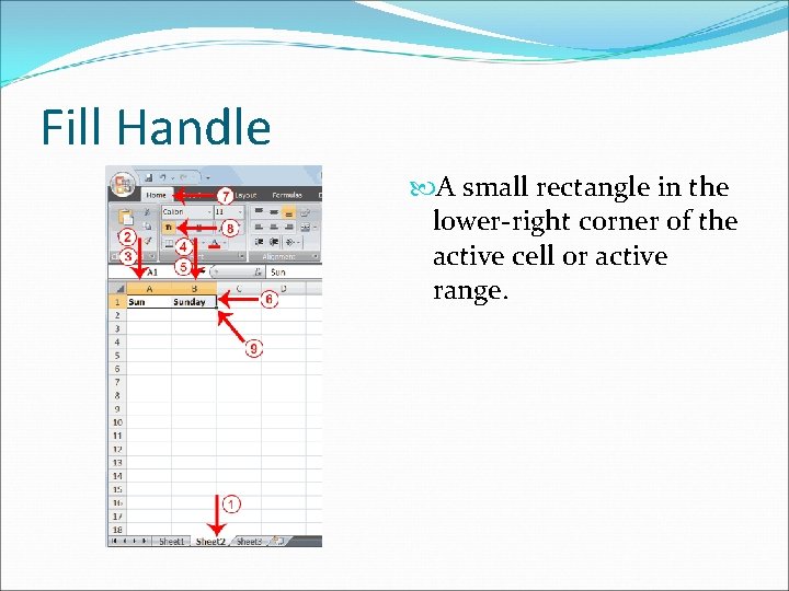
Fill Handle A small rectangle in the lower-right corner of the active cell or active range.
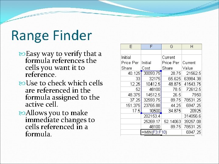
Range Finder Easy way to verify that a formula references the cells you want it to reference. Use to check which cells are referenced in the formula assigned to the active cell. Allows you to make immediate changes to cells referenced in a formula.
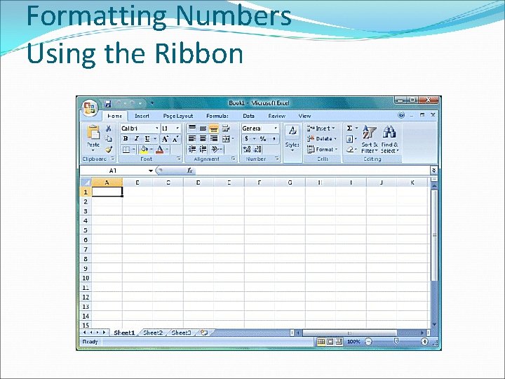
Formatting Numbers Using the Ribbon
Accounting Number Format To add a dollar sign to a number, you should use the Accounting number format. Shows a dollar sign to the left of the number, inserts a comma every three places to the left of the decimal point Displays numbers to the nearest cent.
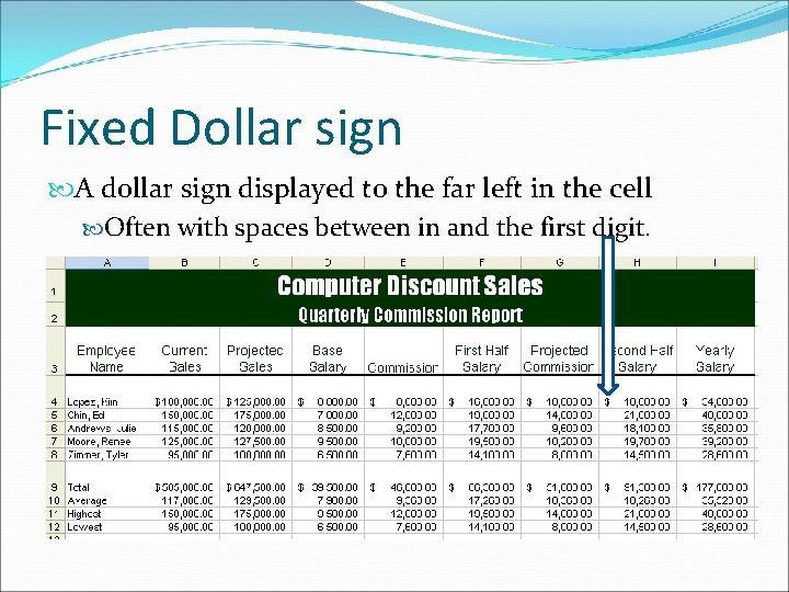
Fixed Dollar sign A dollar sign displayed to the far left in the cell Often with spaces between in and the first digit.
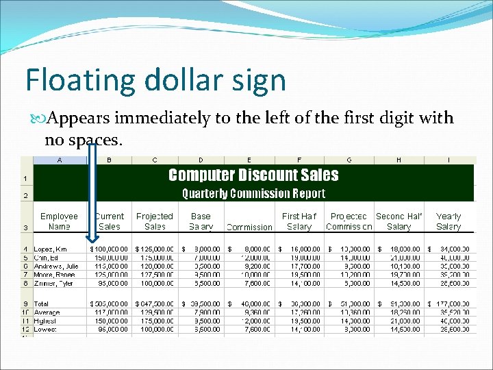
Floating dollar sign Appears immediately to the left of the first digit with no spaces.
Comma Style Format Used to tell Excel to show numbers with commas and no dollar sign. Can be assigned to a range of cells by clicking the Comma Style button Inserts a comma every 3 spaces to the left of the decimal point Causes numbers to be displayed to the nearest 100 ths.
Best fit or Auto adjust The width of the column will increase or decrease so the widest entry will fit in the column. #### in a column means the column is too narrow.
Merging Cells Creating a single cell by combining two or more selected cells. Select the cell range Click the Merge and Center button Worksheet titles and subtitles are usually merged and centered over a worksheet.
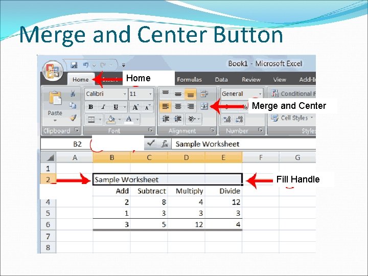
Merge and Center Button Home Merge and Center Fill Handle
Printing the Worksheet Use print preview Turn on gridlines—I want them to show Create a header for the class Print in landscape
Values Version of Worksheet Shows the results of the formulas you have entered Doesn’t show actual formulas used.
Formulas Version Shows the actual formula you have entered Press CTRL + ACCENT MARK (` ) Useful for debugging a worksheet.

Questions?
- Slides: 85