Microsoft Excel 2016 Lesson 7 Formatting Worksheets 2016

Microsoft Excel 2016 Lesson 7 Formatting Worksheets © 2016, John Wiley & Sons, Inc. Microsoft Official Academic Course, Microsoft Excel Core 2016 1

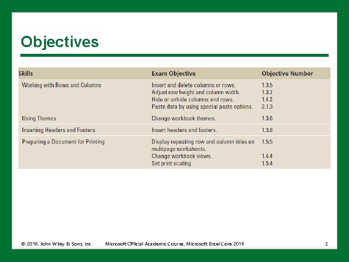
Objectives © 2016, John Wiley & Sons, Inc. Microsoft Official Academic Course, Microsoft Excel Core 2016 2

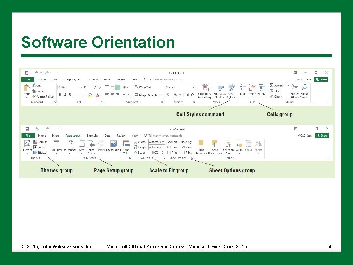
Software Orientation • Excel 2016 provides tools to enhance the look of your worksheets onscreen and in print. • To improve how a worksheet displays or to prepare a worksheet for printing, use commands on the Home tab and the Page Layout tab shown on the next slide. • Use these formatting options to ensure that your worksheets are more useful, more readable, and more attractive. © 2016, John Wiley & Sons, Inc. Microsoft Official Academic Course, Microsoft Excel Core 2016 3

Software Orientation © 2016, John Wiley & Sons, Inc. Microsoft Official Academic Course, Microsoft Excel Core 2016 4

Working with Rows and Columns In Excel, you can: • Insert or delete rows and columns in an existing worksheet • Increase or decrease row height and column width • Hide and unhide rows and columns • Transpose data so that data in a row appears in a column and vice versa. © 2016, John Wiley & Sons, Inc. Microsoft Official Academic Course, Microsoft Excel Core 2016 5

Inserting or Deleting a Row or Column • You will often need to insert additional rows or columns into a worksheet. • To insert a row, select the row or a cell in the row below which you want the new row to appear. The new row is then inserted above the selected cell or row. • To insert multiple rows, select the same number of rows as you want to insert. • Inserting columns works the same way, except columns are inserted to the left of the selected cell or column. • By default, the inserted column is formatted the same as the column to the left. • To deleting a row or column, right-click the row number or column letter and click Delete in the shortcut menu. © 2016, John Wiley & Sons, Inc. Microsoft Official Academic Course, Microsoft Excel Core 2016 6

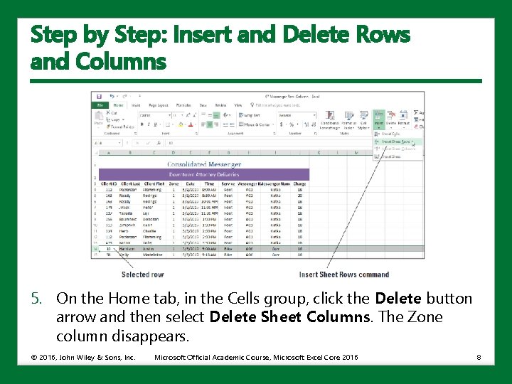
Step by Step: Insert and Delete Rows and Columns 1. OPEN the workbook named 07 Messenger Row-Column. 2. Click the row 14 heading to select the entire row. 3. On the Home tab, in the Cells group, click the Insert button arrow and then select Insert Sheet Rows, as shown in the figure on the next slide. A new blank row appears as row 14. 4. To insert several rows at once, click the row 25 heading, hold down the Ctrl key, and then click row headings 34 and 43. Right-click any of the selected rows and then select Insert from the shortcut menu. Blank rows appear above the selected rows, so that data for each messenger is separated by a blank row. © 2016, John Wiley & Sons, Inc. Microsoft Official Academic Course, Microsoft Excel Core 2016 7

Step by Step: Insert and Delete Rows and Columns 5. On the Home tab, in the Cells group, click the Delete button arrow and then select Delete Sheet Columns. The Zone column disappears. © 2016, John Wiley & Sons, Inc. Microsoft Official Academic Course, Microsoft Excel Core 2016 8

Step by Step: Insert and Delete Rows and Columns 6. Right-click the row 3 heading and select Insert from the shortcut menu. In cell A 3, type Zone 1. 7. Select A 3: I 3. On the Home tab, in the Alignment group, click the Merge & Center button. The “Zone 1” text is centered across the data columns. 8. SAVE the workbook in your Excel Lesson 7 folder as 07 Messenger Row. Column Solution. • LEAVE the workbook open to use in the next exercise. • The column heading or row heading is its identifying letter or number. • You select an entire column or row by clicking its heading. • To select multiple adjacent columns or rows, click the first column or row heading, hold the Shift key, and then click the last heading. • To select multiple nonadjacent columns or rows, click the first column or row heading, and then hold down the Ctrl key while clicking other headings. © 2016, John Wiley & Sons, Inc. Microsoft Official Academic Course, Microsoft Excel Core 2016 9

Modifying Row Height and Column Width • By default, all columns in a new worksheet are the same width and all rows are the same height. • Modifying the height of rows and width of columns can make a worksheet’s contents easier to read and increase its visual appeal. • You can set a row or column to a specific height or width or change the height or width to fit the contents. • To change height and width settings: • Use the Format commands in the Cells group on the Home tab • Use the shortcut menu that appears when you right-click a selected row or column • Double-click or drag the boundary, which is the line between rows or columns. © 2016, John Wiley & Sons, Inc. Microsoft Official Academic Course, Microsoft Excel Core 2016 10

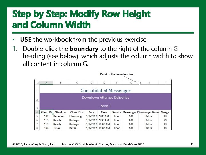
Step by Step: Modify Row Height and Column Width • USE the workbook from the previous exercise. 1. Double-click the boundary to the right of the column G heading (see below), which adjusts the column width to show all content in column G. © 2016, John Wiley & Sons, Inc. Microsoft Official Academic Course, Microsoft Excel Core 2016 11

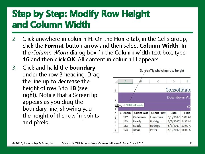
Step by Step: Modify Row Height and Column Width 2. 3. Click anywhere in column H. On the Home tab, in the Cells group, click the Format button arrow and then select Column Width. In the Column Width dialog box, in the Column width text box, type 16 and then click OK. All content in column H appears. Click and hold the boundary under the row 3 heading. Drag the line up to decrease the height of row 3 to 18 (see right). Notice that a Screen. Tip appears as you drag the boundary line, showing you the height of the row in points and pixels. © 2016, John Wiley & Sons, Inc. Microsoft Official Academic Course, Microsoft Excel Core 2016 12

Step by Step: Modify Row Height and Column Width 4. Select row 2. On the Home tab, in the Cells group, click the Format button arrow and then select Auto. Fit Row Height. With the row still selected, click the Format button arrow again and then select Row Height. The Row Height dialog box indicates that the row is 18. 75 points in height. Click OK. 5. SAVE the workbook. • LEAVE the workbook open to use in the next exercise. © 2016, John Wiley & Sons, Inc. Microsoft Official Academic Course, Microsoft Excel Core 2016 13

Step by Step: Modify Row Height and Column Width • Row height (top-to-bottom measurement of a row) is measured in points; one point is equal to 1/72 inch. The default row height is 15 points, but you can specify a row height of 0 to 409 points. • Column width (left-to-right measurement of a column). Although you can specify a column width of 0 to 255 characters, the default column width is 8. 43 characters (based on the default font and font size). If a column width or row height is set to 0, the corresponding column or row is hidden. • If the value entered in a column exceeds the column width, the #### symbols appear, which indicate the number is larger than the column width. © 2016, John Wiley & Sons, Inc. Microsoft Official Academic Course, Microsoft Excel Core 2016 14

Step by Step: Modify Row Height and Column Width • If worksheet data appears crowded or too loose when you use the Auto. Fit Column Width, you can use the mouse to drag the right column boundary for any columns that seem crowded or have too much white space. • White space is the empty area of a document, in which no content appears. • To change the default width for all columns on a worksheet or a workbook, click Format and then select Default Width. • In the Standard Width dialog box, type a new default column measurement. Note that when changing the default column width or row height, columns and rows that contain data or that have been previously formatted retain their formatting. © 2016, John Wiley & Sons, Inc. Microsoft Official Academic Course, Microsoft Excel Core 2016 15

Hiding or Unhiding a Row or Column • If a worksheet contains a large number of rows or columns, you can hide a row or a column using the Hide command or by setting the row height or column width to zero. • When rows are hidden, they do not appear onscreen or in printouts, but the data remains and can be unhidden. © 2016, John Wiley & Sons, Inc. Microsoft Official Academic Course, Microsoft Excel Core 2016 16

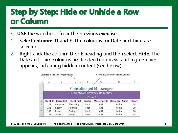
Step by Step: Hide or Unhide a Row or Column • USE the workbook from the previous exercise. 1. Select columns D and E. The columns for Date and Time are selected. 2. Right-click the column D or E heading and then select Hide. The Date and Time columns are hidden from view, and a green line appears, indicating hidden content (see below). © 2016, John Wiley & Sons, Inc. Microsoft Official Academic Course, Microsoft Excel Core 2016 17

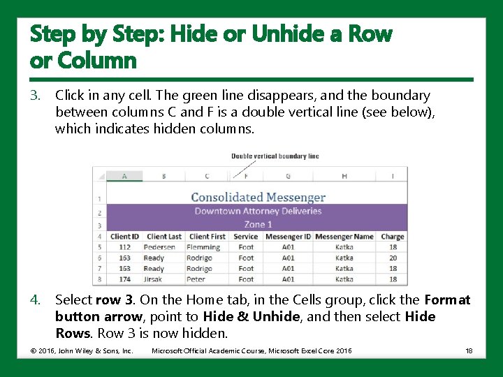
Step by Step: Hide or Unhide a Row or Column 3. Click in any cell. The green line disappears, and the boundary between columns C and F is a double vertical line (see below), which indicates hidden columns. 4. Select row 3. On the Home tab, in the Cells group, click the Format button arrow, point to Hide & Unhide, and then select Hide Rows. Row 3 is now hidden. © 2016, John Wiley & Sons, Inc. Microsoft Official Academic Course, Microsoft Excel Core 2016 18

Step by Step: Hide or Unhide a Row or Column 5. Select rows 2 and 4. Right-click the selection and select Unhide. Row 3 is now visible. 6. SAVE the workbook. • LEAVE the workbook open to use in the next exercise. • To unhide hidden rows, select the row above and the row below the hidden row or rows and use the Unhide Rows command. • To display hidden columns, select the adjacent columns and follow the same steps used for displaying hidden rows. • Use the Go To feature to find a hidden row or column and then make it visible. © 2016, John Wiley & Sons, Inc. Microsoft Official Academic Course, Microsoft Excel Core 2016 19

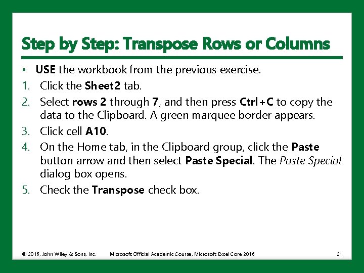
Transposing Rows or Columns • Transposing a row or column causes your cell data to change orientation. • Row data will become column data, and column data will become row data. • Use the Paste Special command to perform this type cell copying. • In the Paste Special dialog box, select the Transpose check box to transpose row or column data. © 2016, John Wiley & Sons, Inc. Microsoft Official Academic Course, Microsoft Excel Core 2016 20

Step by Step: Transpose Rows or Columns • USE the workbook from the previous exercise. 1. Click the Sheet 2 tab. 2. Select rows 2 through 7, and then press Ctrl+C to copy the data to the Clipboard. A green marquee border appears. 3. Click cell A 10. 4. On the Home tab, in the Clipboard group, click the Paste button arrow and then select Paste Special. The Paste Special dialog box opens. 5. Check the Transpose check box. © 2016, John Wiley & Sons, Inc. Microsoft Official Academic Course, Microsoft Excel Core 2016 21

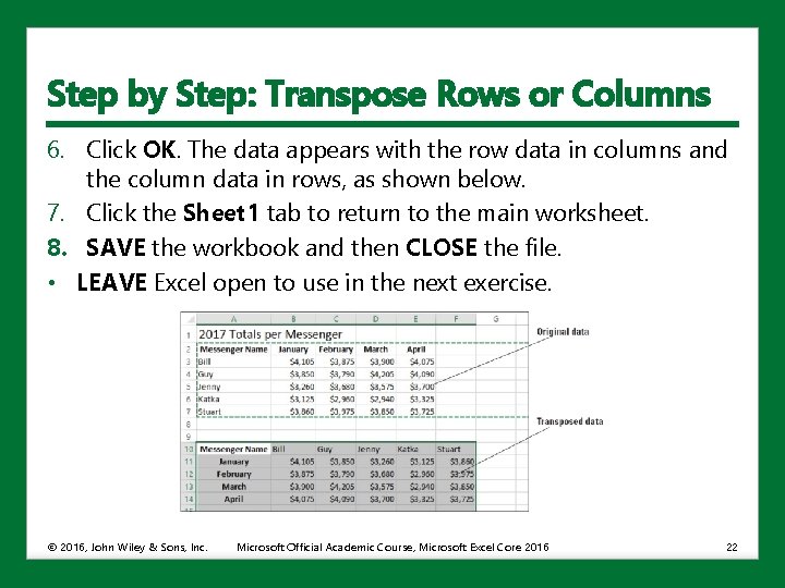
Step by Step: Transpose Rows or Columns 6. Click OK. The data appears with the row data in columns and the column data in rows, as shown below. 7. Click the Sheet 1 tab to return to the main worksheet. 8. SAVE the workbook and then CLOSE the file. • LEAVE Excel open to use in the next exercise. © 2016, John Wiley & Sons, Inc. Microsoft Official Academic Course, Microsoft Excel Core 2016 22

Using Themes • A document theme is a predefined set of colors, fonts, and effects that can be applied to a workbook. • Use document themes to easily format an entire document. • Themes are used in other Office applications so you can give all your Office documents a uniform look in terms of colors, fonts, and effects. • Effects, such as shadows or bevels, modify the appearance of an object. • Excel has several predefined document themes. • When you apply a theme to a workbook, the colors, fonts, and effects contained within that theme replace any styles that were already applied to cells or ranges. © 2016, John Wiley & Sons, Inc. Microsoft Official Academic Course, Microsoft Excel Core 2016 23

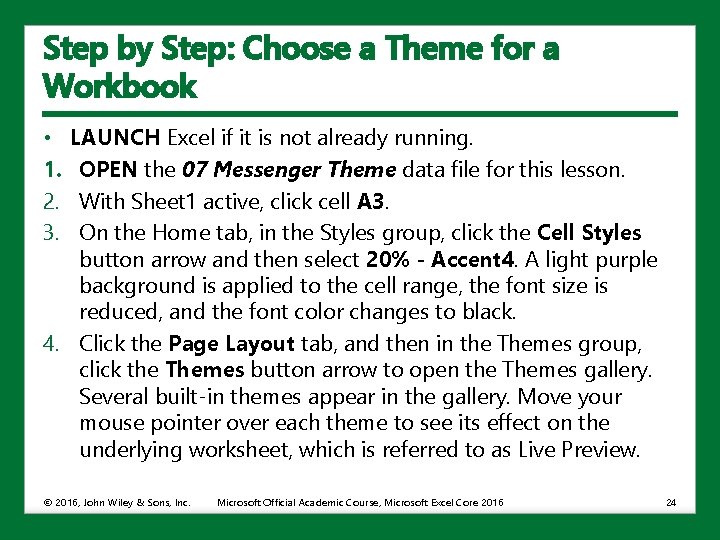
Step by Step: Choose a Theme for a Workbook • 1. 2. 3. LAUNCH Excel if it is not already running. OPEN the 07 Messenger Theme data file for this lesson. With Sheet 1 active, click cell A 3. On the Home tab, in the Styles group, click the Cell Styles button arrow and then select 20% - Accent 4. A light purple background is applied to the cell range, the font size is reduced, and the font color changes to black. 4. Click the Page Layout tab, and then in the Themes group, click the Themes button arrow to open the Themes gallery. Several built-in themes appear in the gallery. Move your mouse pointer over each theme to see its effect on the underlying worksheet, which is referred to as Live Preview. © 2016, John Wiley & Sons, Inc. Microsoft Official Academic Course, Microsoft Excel Core 2016 24

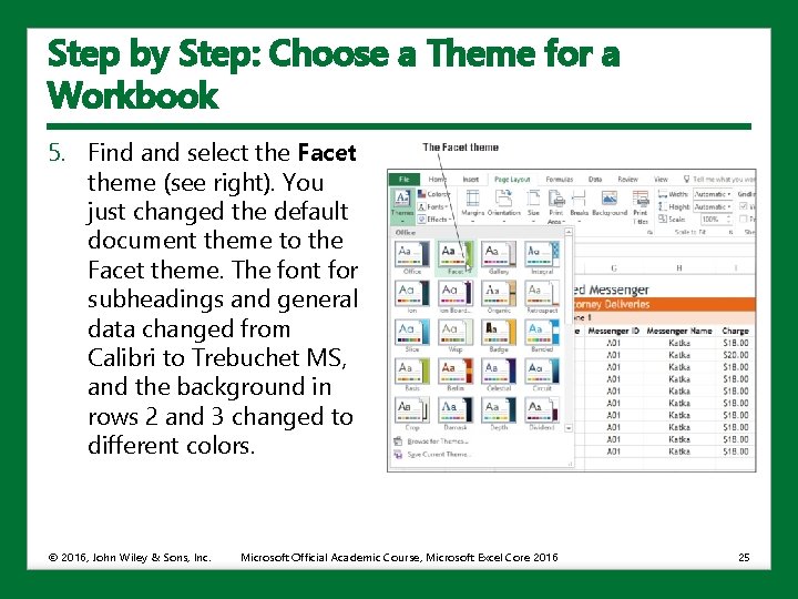
Step by Step: Choose a Theme for a Workbook 5. Find and select the Facet theme (see right). You just changed the default document theme to the Facet theme. The font for subheadings and general data changed from Calibri to Trebuchet MS, and the background in rows 2 and 3 changed to different colors. © 2016, John Wiley & Sons, Inc. Microsoft Official Academic Course, Microsoft Excel Core 2016 25

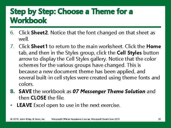
Step by Step: Choose a Theme for a Workbook 6. Click Sheet 2. Notice that the font changed on that sheet as well. 7. Click Sheet 1 to return to the main worksheet. Click the Home tab, and then in the Styles group, click the Cell Styles button arrow to display the Cell Styles gallery. Notice that the color schemes for the various groups have changed. This is because a new document theme has been applied, and several built-in cell styles were created using theme fonts and colors. 8. SAVE the workbook as 07 Messenger Theme Solution and then CLOSE the file. • LEAVE Excel open to use in the next exercise. © 2016, John Wiley & Sons, Inc. Microsoft Official Academic Course, Microsoft Excel Core 2016 26

Step by Step: Choose a Theme for a Workbook • Applying a new theme changes fonts and colors, and the color of shapes and Smart. Art, tables, charts, and other objects. • Cell styles are used to format specific cells or ranges within a worksheet; document themes are used to apply sets of styles (colors, fonts, and fill effects) to an entire document. • Many built-in cell styles use theme-aware formatting, so applying a new theme determines which fonts and colors are used by styles. • Styles are independent from themes in that you can change styles regardless of theme that’s applied to a document. © 2016, John Wiley & Sons, Inc. Microsoft Official Academic Course, Microsoft Excel Core 2016 27

Viewing and Printing Worksheet Gridlines • Worksheet gridlines (the lines that display around worksheet cells), row headings, and column headings can be used to enhance a worksheet’s appearance. • Gridlines appear onscreen, by default, but are not printed automatically. • You can choose to show or hide gridlines in your worksheet • You can choose whether gridlines are printed. A printed worksheet is easier to read when gridlines are included. © 2016, John Wiley & Sons, Inc. Microsoft Official Academic Course, Microsoft Excel Core 2016 28

Step by Step: View and Print a Worksheet’s Gridlines • LAUNCH Excel if it is not already running. 1. OPEN 07 Messenger Appearance and ensure Sheet 1 is active. 2. Click the Page Layout tab, and then in the Sheet Options group, uncheck the Gridlines View check box. The gridlines disappear from the worksheet. 3. Check the Gridlines View check box to restore viewable gridlines. 4. Check the Gridlines Print check box. This action will force gridlines to appear in your printed worksheet. 5. Click the Dialog Box Launcher in the Sheet Options group to open the Page Setup dialog box. © 2016, John Wiley & Sons, Inc. Microsoft Official Academic Course, Microsoft Excel Core 2016 29

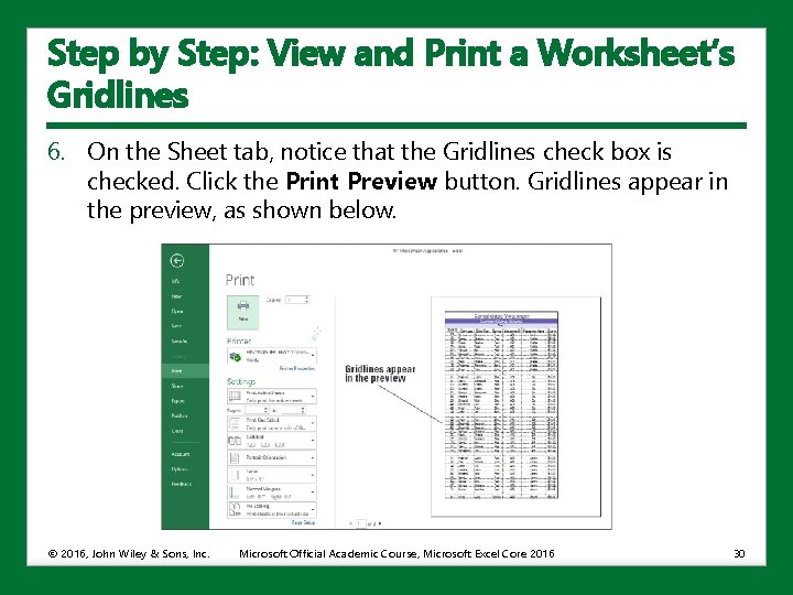
Step by Step: View and Print a Worksheet’s Gridlines 6. On the Sheet tab, notice that the Gridlines check box is checked. Click the Print Preview button. Gridlines appear in the preview, as shown below. © 2016, John Wiley & Sons, Inc. Microsoft Official Academic Course, Microsoft Excel Core 2016 30

Step by Step: View and Print a Worksheet’s Gridlines 7. In the upper-left corner of the Print window, click the Return to document button to return to the worksheet. 8. SAVE the workbook as 07 Messenger Appearance Solution and then CLOSE the file. • LEAVE Excel open to use in the next exercise. • Print Preview is the screen that appears when you click the File tab and then click Print, or if you click Print Preview in a dialog box that provides the button. • Print Preview allows you to see what your document will look like before you print it. © 2016, John Wiley & Sons, Inc. Microsoft Official Academic Course, Microsoft Excel Core 2016 31

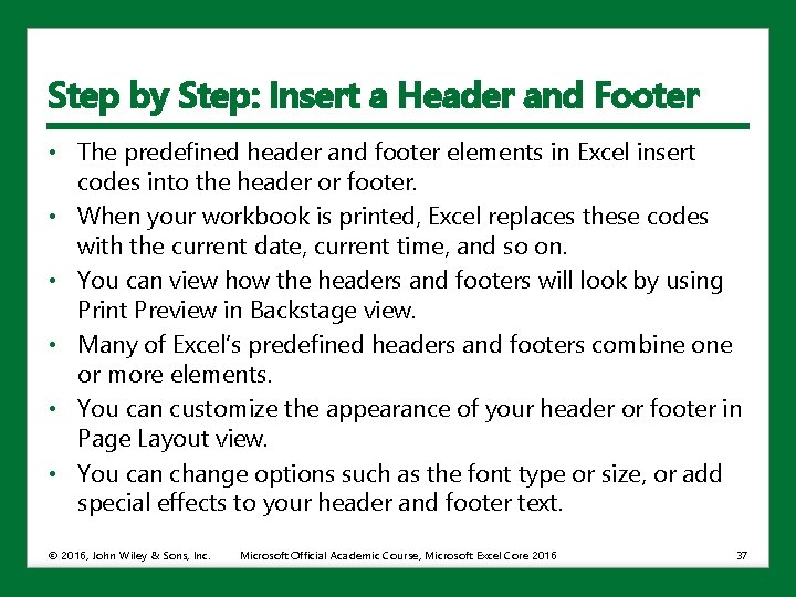
Inserting Headers and Footers • Headers or footers provide useful information about the worksheet, such as who prepared it, the date it was created or last modified, the page number, and so on. • Headers and footers are visible in Page Layout view and appear on printouts. • A header is a line of text that appears at the top of each page of a printed worksheet. • A footer is a line of text that appears at the bottom of each page. © 2016, John Wiley & Sons, Inc. Microsoft Official Academic Course, Microsoft Excel Core 2016 32

Inserting Headers and Footers • You can: • Add predefined header or footer information to a worksheet • Insert elements such as page numbers, date and time, and filename • Add your own content to a header or footer. • On the Header & Footer Tools Design tab, the Header & Footer group contains predefined headers and footers that allow you to automatically add text to the header or footer. • You also can create a custom header or footer by manually typing the text you want to include. © 2016, John Wiley & Sons, Inc. Microsoft Official Academic Course, Microsoft Excel Core 2016 33

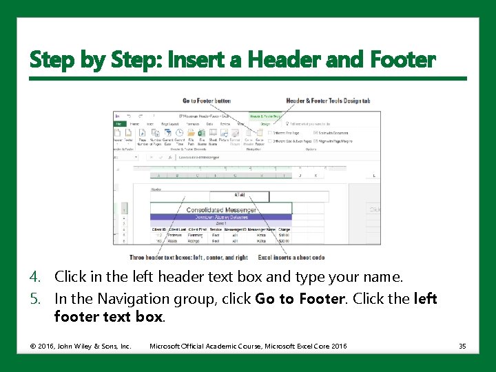
Step by Step: Insert a Header and Footer • LAUNCH Excel if it is not already running. 1. OPEN 07 Messenger Header-Footer and ensure Sheet 1 is active. Click cell A 1. 2. Click the View tab, and then in the Workbook Views group, click the Page Layout button to view headers and footers. 3. Click the center header text box (which displays the “Add header” placeholder text). Click the Header & Footer Tools Design tab now that it has become active. In the Header & Footer Elements group, click Sheet Name. The code &[Tab] appears in the text box (see the figure on the next slide). © 2016, John Wiley & Sons, Inc. Microsoft Official Academic Course, Microsoft Excel Core 2016 34

Step by Step: Insert a Header and Footer 4. Click in the left header text box and type your name. 5. In the Navigation group, click Go to Footer. Click the left footer text box. © 2016, John Wiley & Sons, Inc. Microsoft Official Academic Course, Microsoft Excel Core 2016 35

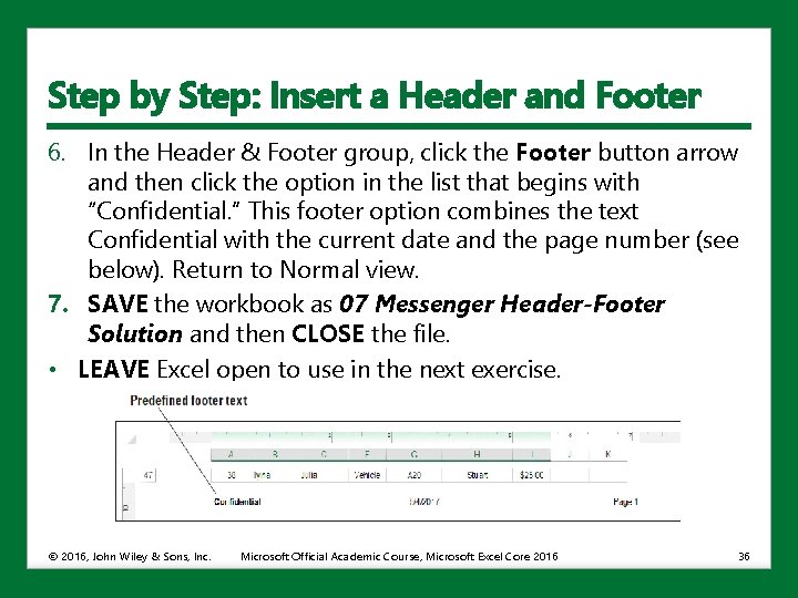
Step by Step: Insert a Header and Footer 6. In the Header & Footer group, click the Footer button arrow and then click the option in the list that begins with “Confidential. ” This footer option combines the text Confidential with the current date and the page number (see below). Return to Normal view. 7. SAVE the workbook as 07 Messenger Header-Footer Solution and then CLOSE the file. • LEAVE Excel open to use in the next exercise. © 2016, John Wiley & Sons, Inc. Microsoft Official Academic Course, Microsoft Excel Core 2016 36

Step by Step: Insert a Header and Footer • The predefined header and footer elements in Excel insert codes into the header or footer. • When your workbook is printed, Excel replaces these codes with the current date, current time, and so on. • You can view how the headers and footers will look by using Print Preview in Backstage view. • Many of Excel’s predefined headers and footers combine or more elements. • You can customize the appearance of your header or footer in Page Layout view. • You can change options such as the font type or size, or add special effects to your header and footer text. © 2016, John Wiley & Sons, Inc. Microsoft Official Academic Course, Microsoft Excel Core 2016 37

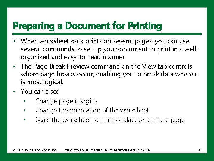
Preparing a Document for Printing • When worksheet data prints on several pages, you can use several commands to set up your document to print in a wellorganized and easy-to-read manner. • The Page Break Preview command on the View tab controls where page breaks occur, enabling you to break data where it is most logical. • You can also: • Change page margins • Change the orientation of the worksheet • Scale the worksheet to fit more data on a single page © 2016, John Wiley & Sons, Inc. Microsoft Official Academic Course, Microsoft Excel Core 2016 38

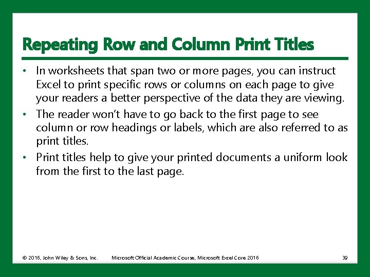
Repeating Row and Column Print Titles • In worksheets that span two or more pages, you can instruct Excel to print specific rows or columns on each page to give your readers a better perspective of the data they are viewing. • The reader won’t have to go back to the first page to see column or row headings or labels, which are also referred to as print titles. • Print titles help to give your printed documents a uniform look from the first to the last page. © 2016, John Wiley & Sons, Inc. Microsoft Official Academic Course, Microsoft Excel Core 2016 39

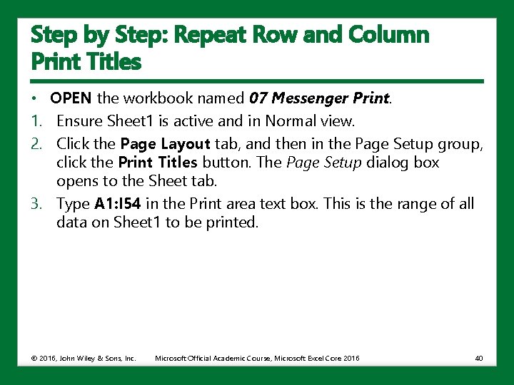
Step by Step: Repeat Row and Column Print Titles • OPEN the workbook named 07 Messenger Print. 1. Ensure Sheet 1 is active and in Normal view. 2. Click the Page Layout tab, and then in the Page Setup group, click the Print Titles button. The Page Setup dialog box opens to the Sheet tab. 3. Type A 1: I 54 in the Print area text box. This is the range of all data on Sheet 1 to be printed. © 2016, John Wiley & Sons, Inc. Microsoft Official Academic Course, Microsoft Excel Core 2016 40

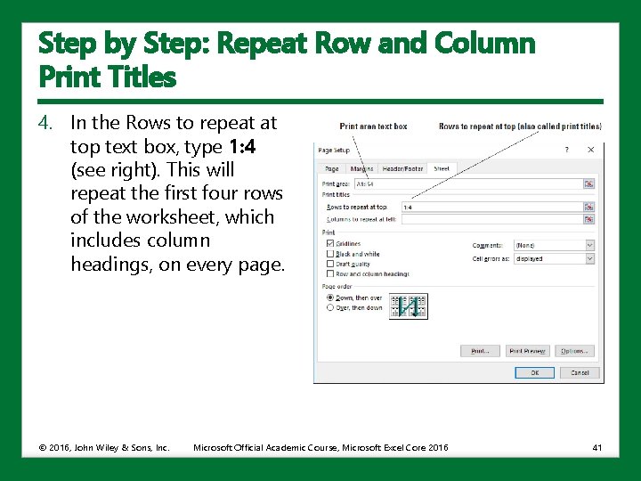
Step by Step: Repeat Row and Column Print Titles 4. In the Rows to repeat at top text box, type 1: 4 (see right). This will repeat the first four rows of the worksheet, which includes column headings, on every page. © 2016, John Wiley & Sons, Inc. Microsoft Official Academic Course, Microsoft Excel Core 2016 41

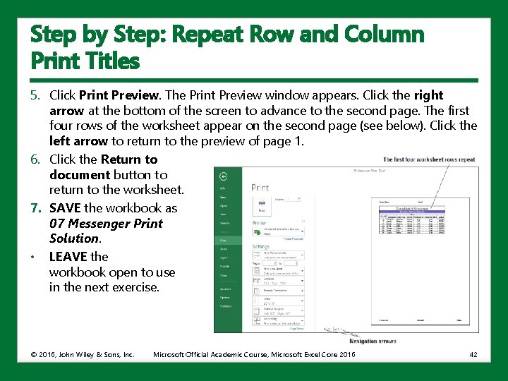
Step by Step: Repeat Row and Column Print Titles 5. Click Print Preview. The Print Preview window appears. Click the right arrow at the bottom of the screen to advance to the second page. The first four rows of the worksheet appear on the second page (see below). Click the left arrow to return to the preview of page 1. 6. Click the Return to document button to return to the worksheet. 7. SAVE the workbook as 07 Messenger Print Solution. • LEAVE the workbook open to use in the next exercise. © 2016, John Wiley & Sons, Inc. Microsoft Official Academic Course, Microsoft Excel Core 2016 42

Adding and Moving a Page Break • The Print window in Backstage view displays a full-page preview of a worksheet just as it will be printed. • With Print Preview, you can check the format and overall layout of a worksheet before actually printing it. • You cannot make changes to the document in Print Preview. • A page break is a divider that breaks a worksheet into separate pages for printing. • Excel inserts automatic vertical page breaks (shown as a broken line) based on paper size, margin settings, scaling options, and the positions of any manual page breaks (shown as a solid line) that you insert. • Excel provides a Page Break Preview window in which you can quickly adjust automatic page breaks to achieve a more desirable printed document. © 2016, John Wiley & Sons, Inc. Microsoft Official Academic Course, Microsoft Excel Core 2016 43

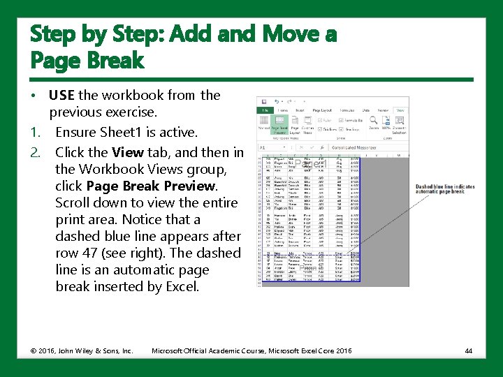
Step by Step: Add and Move a Page Break • USE the workbook from the previous exercise. 1. Ensure Sheet 1 is active. 2. Click the View tab, and then in the Workbook Views group, click Page Break Preview. Scroll down to view the entire print area. Notice that a dashed blue line appears after row 47 (see right). The dashed line is an automatic page break inserted by Excel. © 2016, John Wiley & Sons, Inc. Microsoft Official Academic Course, Microsoft Excel Core 2016 44

Step by Step: Add and Move a Page Break 3. 4. 5. • • • Click and hold the horizontal automatic page break and drag it upward so it is now just below row 46. The automatic page break is now a manual page break represented by a solid blue line. On the View tab, in the Workbook Views group, click Normal. SAVE the workbook. LEAVE the workbook open to use in the next exercise. Use manual page breaks to control page break locations. You can drag an automatic page break to a new location to convert it to a manual page break. Or click a cell in the row where you want a page break to occur, then click the Page Layout tab. In the Page Setup group, click Breaks and then Insert Page Break. A horizontal page break appears. © 2016, John Wiley & Sons, Inc. Microsoft Official Academic Course, Microsoft Excel Core 2016 45

Step by Step: Set Margins • Margins are an effective way to manage and optimize the white space on a printed worksheet • In Excel, you can choose one of three built-in margin sets, or you can create custom margins using the Page Setup dialog box. • USE the workbook from the previous exercise. 1. Ensure Sheet 1 is active and in Normal view. 2. Click the Page Layout tab, and then in the Page Setup group, click the Margins button arrow to open the Margins menu. © 2016, John Wiley & Sons, Inc. Microsoft Official Academic Course, Microsoft Excel Core 2016 46

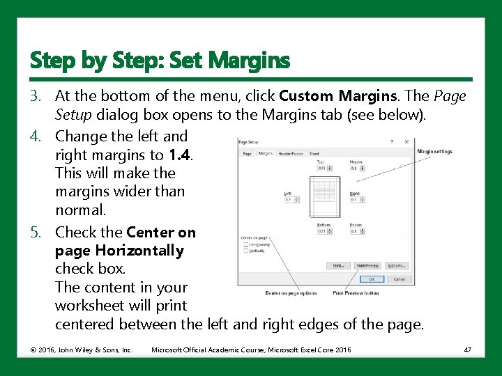
Step by Step: Set Margins 3. At the bottom of the menu, click Custom Margins. The Page Setup dialog box opens to the Margins tab (see below). 4. Change the left and right margins to 1. 4. This will make the margins wider than normal. 5. Check the Center on page Horizontally check box. The content in your worksheet will print centered between the left and right edges of the page. © 2016, John Wiley & Sons, Inc. Microsoft Official Academic Course, Microsoft Excel Core 2016 47

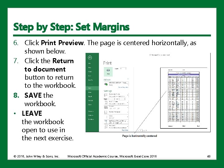
Step by Step: Set Margins 6. Click Print Preview. The page is centered horizontally, as shown below. 7. Click the Return to document button to return to the workbook. 8. SAVE the workbook. • LEAVE the workbook open to use in the next exercise. © 2016, John Wiley & Sons, Inc. Microsoft Official Academic Course, Microsoft Excel Core 2016 48

Step by Step: Set Margins • • The Margins menu includes the following predefined settings: • Normal margin setting is the default for a new workbook. • Narrow margins allow more area for data when you print a workbook • Wider margins introduce more white space. You can also set custom margins in Excel. When you click Custom Margins, the Page Setup dialog box opens with the settings that have been applied to the active worksheet. You can change any of the settings to create a custom margin setting. Header and footer margins automatically adjust when you change the page margins. Worksheets that do not fill an entire page can be centered vertically and horizontally using the Margins tab of the Page Setup dialog box. On the Page Layout tab, in the Page Setup group, click the Breaks button arrow and then select Reset All Page Breaks to quickly remove all manual page breaks from a worksheet. © 2016, John Wiley & Sons, Inc. Microsoft Official Academic Course, Microsoft Excel Core 2016 49

Setting a Worksheet’s Orientation • Printed worksheets are easiest to read analyze when all of the data appears on one piece of paper. • Excel’s orientation and scaling features give you control over the number of printed pages of worksheet data. • You can change the orientation of a worksheet, which is the position of the content. • A worksheet printed vertically uses the Portrait orientation, which is the default setting. • A worksheet printed horizontally uses the Landscape orientation. © 2016, John Wiley & Sons, Inc. Microsoft Official Academic Course, Microsoft Excel Core 2016 50

Step by Step: Set a Worksheet’s Orientation • USE the workbook from the previous exercise. 1. Ensure Sheet 1 is active and in Normal view. 2. On the Page Layout tab, in the Page Setup group, click Orientation and then click Landscape. 3. Click the File tab, and then click Print. Click through the pages to see the worksheet in Landscape orientation. If you decided to keep this orientation, you would need to adjust page breaks to display all content properly. 4. Click the Return to document button to return to the workbook. 5. Repeat Step 2 to change the orientation back to Portrait. 6. SAVE the workbook. • LEAVE the workbook open to use in the next exercise. © 2016, John Wiley & Sons, Inc. Microsoft Official Academic Course, Microsoft Excel Core 2016 51

Scaling a Worksheet to Fit on a Printed Page • Scaling refers to shrinking or stretching printed output to a percentage of its actual size. • One use for scaling is to resize a document so that it fits on a single page. • Before attempting to change the scaling for a worksheet’s output, the maximum width and height must be set to Automatic. © 2016, John Wiley & Sons, Inc. Microsoft Official Academic Course, Microsoft Excel Core 2016 52

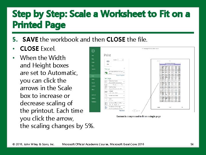
Step by Step: Scale a Worksheet to Fit on a Printed Page • USE the workbook from the previous exercise. 1. Ensure Sheet 1 is active and in Normal view. 2. On the Page Layout tab, in the Page Setup group, click Orientation and verify that Portrait is selected. 3. In the Scale to Fit group, click the Height arrow and then select 1 page. The scale of the worksheet is reduced so that all rows fit on the same page. 4. Click the File tab, and then click Print. Notice that all rows appear on the page and that the content is smaller than it was previously, as shown in the figure on the next slide. When output is reduced, it shrinks the height and width proportionally. © 2016, John Wiley & Sons, Inc. Microsoft Official Academic Course, Microsoft Excel Core 2016 53

Step by Step: Scale a Worksheet to Fit on a Printed Page 5. SAVE the workbook and then CLOSE the file. • CLOSE Excel. • When the Width and Height boxes are set to Automatic, you can click the arrows in the Scale box to increase or decrease scaling of the printout. Each time you click the arrow, the scaling changes by 5%. © 2016, John Wiley & Sons, Inc. Microsoft Official Academic Course, Microsoft Excel Core 2016 54

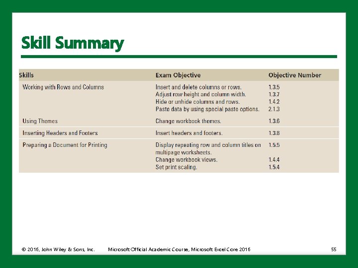
Skill Summary © 2016, John Wiley & Sons, Inc. Microsoft Official Academic Course, Microsoft Excel Core 2016 55