Microsoft Excel 2016 Lesson 5 Using Functions 2016

Microsoft Excel 2016 Lesson 5 Using Functions © 2016, John Wiley & Sons, Inc. Microsoft Official Academic Course, Microsoft Excel Core 2016 1

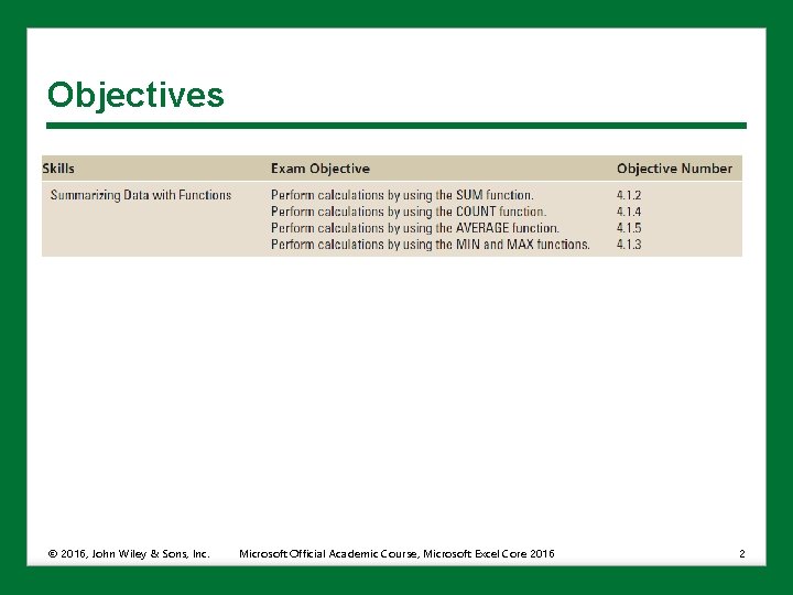
Objectives © 2016, John Wiley & Sons, Inc. Microsoft Official Academic Course, Microsoft Excel Core 2016 2

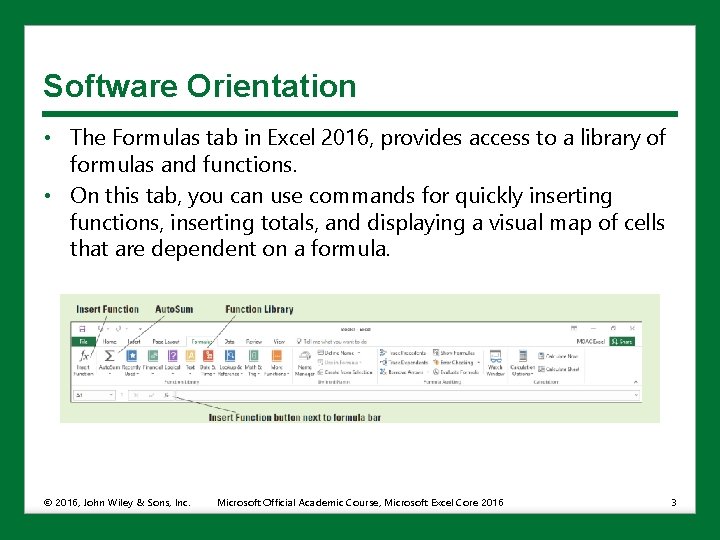
Software Orientation • The Formulas tab in Excel 2016, provides access to a library of formulas and functions. • On this tab, you can use commands for quickly inserting functions, inserting totals, and displaying a visual map of cells that are dependent on a formula. © 2016, John Wiley & Sons, Inc. Microsoft Official Academic Course, Microsoft Excel Core 2016 3

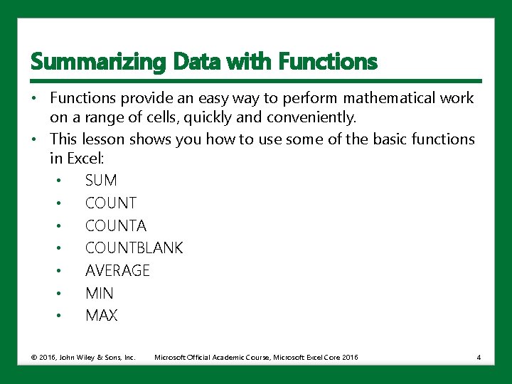
Summarizing Data with Functions • Functions provide an easy way to perform mathematical work on a range of cells, quickly and conveniently. • This lesson shows you how to use some of the basic functions in Excel: • SUM • COUNTA • COUNTBLANK • AVERAGE • MIN • MAX © 2016, John Wiley & Sons, Inc. Microsoft Official Academic Course, Microsoft Excel Core 2016 4

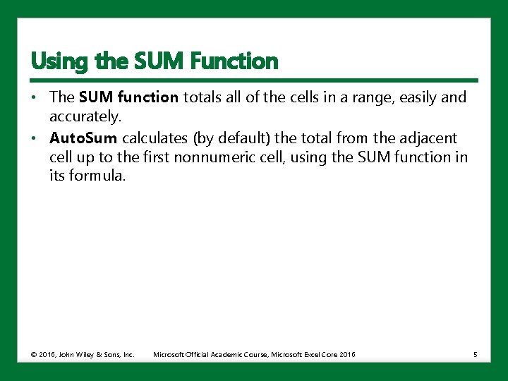
Using the SUM Function • The SUM function totals all of the cells in a range, easily and accurately. • Auto. Sum calculates (by default) the total from the adjacent cell up to the first nonnumeric cell, using the SUM function in its formula. © 2016, John Wiley & Sons, Inc. Microsoft Official Academic Course, Microsoft Excel Core 2016 5

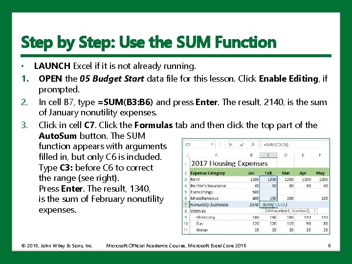
Step by Step: Use the SUM Function • LAUNCH Excel if it is not already running. 1. OPEN the 05 Budget Start data file for this lesson. Click Enable Editing, if prompted. 2. In cell B 7, type =SUM(B 3: B 6) and press Enter. The result, 2140, is the sum of January nonutility expenses. 3. Click in cell C 7. Click the Formulas tab and then click the top part of the Auto. Sum button. The SUM function appears with arguments filled in, but only C 6 is included. Type C 3: before C 6 to correct the range (see right). Press Enter. The result, 1340, is the sum of February nonutility expenses. © 2016, John Wiley & Sons, Inc. Microsoft Official Academic Course, Microsoft Excel Core 2016 6

Step by Step: Use the SUM Function 4. Copy cell C 7 to D 7: M 7 to enter the remaining subtotals. 5. Copy cell N 6 to N 7 to enter the total nonutility expenses. 6. SAVE the workbook to your Excel Lesson 5 folder as 05 Budget Math Solution. • LEAVE the workbook open. • The alternative to the SUM function is to create an addition formula using cell references for every cell value to be added: =B 7+C 7+D 7+E 7+F 7+G 7+H 7+I 7+J 7+K 7+L 7+M 7 • It’s easier to use the SUM function or Auto. Sum. • Auto. Sum is a built-in feature of Excel that recognizes adjacent cells in rows and columns as the logical selection to perform the Auto. Sum. © 2016, John Wiley & Sons, Inc. Microsoft Official Academic Course, Microsoft Excel Core 2016 7

Using the COUNT, COUNTA, and COUNTBLANK Functions • Statistical functions, such as SUM and COUNT, compile and classify data to present significant information. • Use the COUNT function when you want to determine how many cells in a range contain a number. • The COUNTA function counts all nonblank entries in a range, whether they include text or numbers. • The COUNTBLANK function counts the number of blank cells in a range. © 2016, John Wiley & Sons, Inc. Microsoft Official Academic Course, Microsoft Excel Core 2016 8

Step by Step: Use the COUNT, COUNTA, and COUNTBLANK Functions • USE the workbook you modified in the previous exercise. 1. In cell O 5, type COUNT and then press Enter. This is the label identifying the formula you will enter in the next step. 2. In cell O 6, type =COUNT(A 6: M 6) and then press Enter. The result, 9, is the number of months in which you budgeted for miscellaneous expenses. The COUNT function disregards the entry in A 6 because it doesn’t contain a number, and the function also disregards blank cells. 3. In cell P 5, type COUNTA and then press Enter. This is the label identifying the formula you will enter in the next step. 4. In cell P 6, type =COUNTA(A 6: M 6) and then press Enter. The result, 10, is the number of nonblank entries in the range. © 2016, John Wiley & Sons, Inc. Microsoft Official Academic Course, Microsoft Excel Core 2016 9

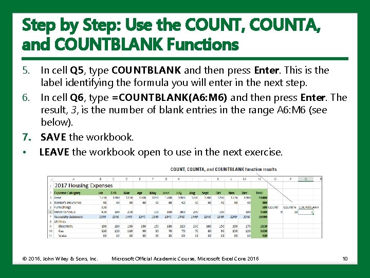
Step by Step: Use the COUNT, COUNTA, and COUNTBLANK Functions 5. In cell Q 5, type COUNTBLANK and then press Enter. This is the label identifying the formula you will enter in the next step. 6. In cell Q 6, type =COUNTBLANK(A 6: M 6) and then press Enter. The result, 3, is the number of blank entries in the range A 6: M 6 (see below). 7. SAVE the workbook. • LEAVE the workbook open to use in the next exercise. © 2016, John Wiley & Sons, Inc. Microsoft Official Academic Course, Microsoft Excel Core 2016 10

Step by Step: Use the AVERAGE Function • The AVERAGE function adds a range of cells and then divides by the number of cell entries, determining the mean value of all values in the range. • USE the workbook you modified in the previous exercise. 1. In cell O 8, type AVERAGE and then press Enter. 2. In cell O 9, type =AVERAGE(B 9: M 9) and then press Enter. The result, 175. 8333, is your average expected monthly electricity bill. © 2016, John Wiley & Sons, Inc. Microsoft Official Academic Course, Microsoft Excel Core 2016 11

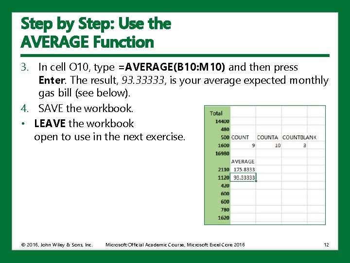
Step by Step: Use the AVERAGE Function 3. In cell O 10, type =AVERAGE(B 10: M 10) and then press Enter. The result, 93. 33333, is your average expected monthly gas bill (see below). 4. SAVE the workbook. • LEAVE the workbook open to use in the next exercise. © 2016, John Wiley & Sons, Inc. Microsoft Official Academic Course, Microsoft Excel Core 2016 12

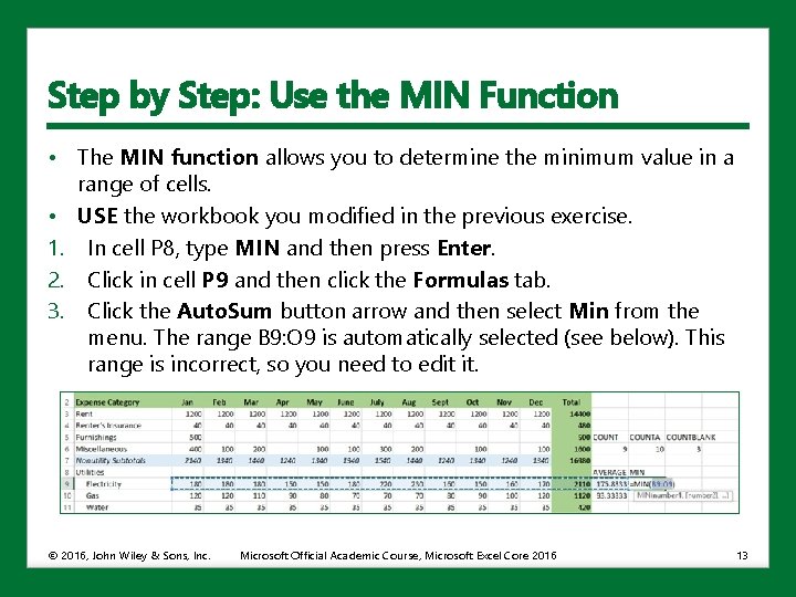
Step by Step: Use the MIN Function • The MIN function allows you to determine the minimum value in a range of cells. • USE the workbook you modified in the previous exercise. 1. In cell P 8, type MIN and then press Enter. 2. Click in cell P 9 and then click the Formulas tab. 3. Click the Auto. Sum button arrow and then select Min from the menu. The range B 9: O 9 is automatically selected (see below). This range is incorrect, so you need to edit it. © 2016, John Wiley & Sons, Inc. Microsoft Official Academic Course, Microsoft Excel Core 2016 13

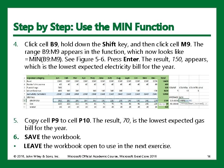
Step by Step: Use the MIN Function 4. Click cell B 9, hold down the Shift key, and then click cell M 9. The range B 9: M 9 appears in the function, which now looks like =MIN(B 9: M 9). See Figure 5 -6. Press Enter. The result, 150, appears, which is the lowest expected electricity bill for the year. 5. Copy cell P 9 to cell P 10. The result, 70, is the lowest expected gas bill for the year. 6. SAVE the workbook. • LEAVE the workbook open to use in the next exercise. © 2016, John Wiley & Sons, Inc. Microsoft Official Academic Course, Microsoft Excel Core 2016 14

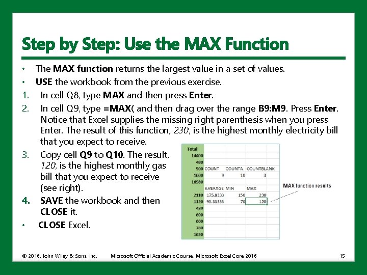
Step by Step: Use the MAX Function • The MAX function returns the largest value in a set of values. • USE the workbook from the previous exercise. 1. In cell Q 8, type MAX and then press Enter. 2. In cell Q 9, type =MAX( and then drag over the range B 9: M 9. Press Enter. Notice that Excel supplies the missing right parenthesis when you press Enter. The result of this function, 230, is the highest monthly electricity bill that you expect to receive. 3. Copy cell Q 9 to Q 10. The result, 120, is the highest monthly gas bill that you expect to receive (see right). 4. SAVE the workbook and then CLOSE it. • CLOSE Excel. © 2016, John Wiley & Sons, Inc. Microsoft Official Academic Course, Microsoft Excel Core 2016 15

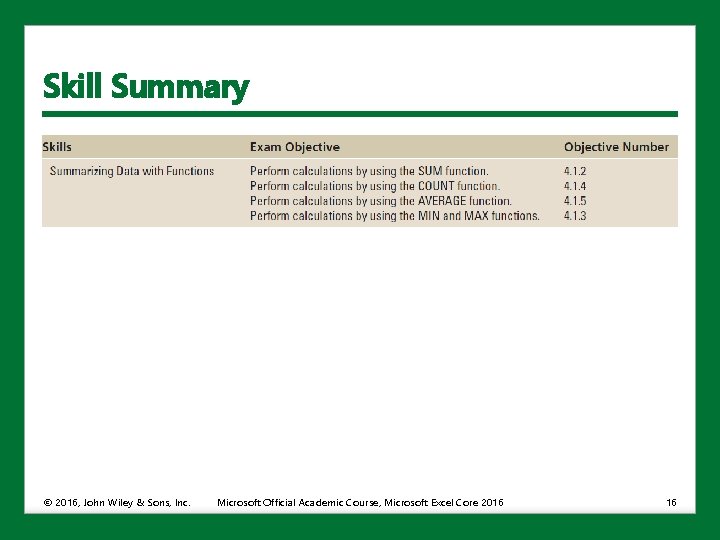
Skill Summary © 2016, John Wiley & Sons, Inc. Microsoft Official Academic Course, Microsoft Excel Core 2016 16