Microsoft Excel 2016 Lesson 2 Working with Microsoft

Microsoft Excel 2016 Lesson 2 Working with Microsoft Excel 2016 © 2016, John Wiley & Sons, Inc. Microsoft Official Academic Course, Microsoft Excel Core 2016 1

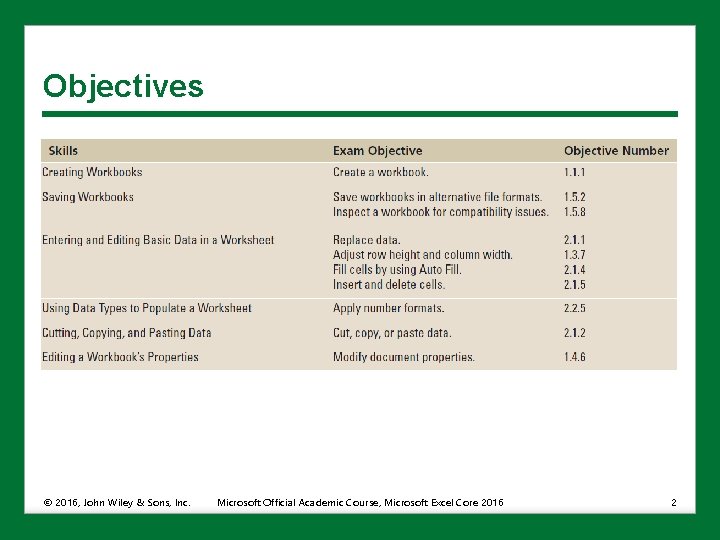
Objectives © 2016, John Wiley & Sons, Inc. Microsoft Official Academic Course, Microsoft Excel Core 2016 2

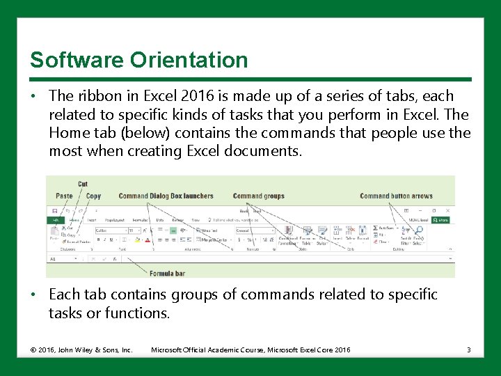
Software Orientation • The ribbon in Excel 2016 is made up of a series of tabs, each related to specific kinds of tasks that you perform in Excel. The Home tab (below) contains the commands that people use the most when creating Excel documents. • Each tab contains groups of commands related to specific tasks or functions. © 2016, John Wiley & Sons, Inc. Microsoft Official Academic Course, Microsoft Excel Core 2016 3

Software Orientation • Commands that have an arrow associated with them (see Auto. Sum and Find & Select in the previous slide) have other options available for the task. • The Dialog Box Launchers in groups display additional commands not shown on the ribbon. • In the figure in the previous slide, the Clipboard, Font, Alignment, and Number groups have associated dialog boxes or task panes, whereas Styles, Cells, and Editing do not. © 2016, John Wiley & Sons, Inc. Microsoft Official Academic Course, Microsoft Excel Core 2016 4

Creating Workbooks • There are three ways to create a new Microsoft Excel workbook. • Open a new, blank workbook when you launch Excel or use the File tab to access Backstage view. • Open an existing Excel workbook, enter new or additional data, and save the file with a new name. • Use a template to create a new workbook. (A template is a model that has already been set up to display certain kinds of data, such as sales reports, invoices, and so on. ) © 2016, John Wiley & Sons, Inc. Microsoft Official Academic Course, Microsoft Excel Core 2016 5

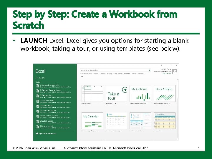
Step by Step: Create a Workbook from Scratch • LAUNCH Excel gives you options for starting a blank workbook, taking a tour, or using templates (see below). © 2016, John Wiley & Sons, Inc. Microsoft Official Academic Course, Microsoft Excel Core 2016 6

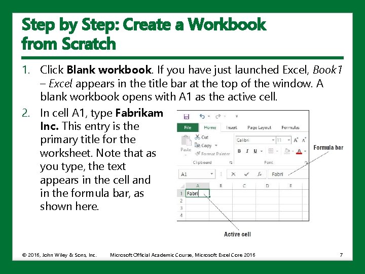
Step by Step: Create a Workbook from Scratch 1. Click Blank workbook. If you have just launched Excel, Book 1 – Excel appears in the title bar at the top of the window. A blank workbook opens with A 1 as the active cell. 2. In cell A 1, type Fabrikam Inc. This entry is the primary title for the worksheet. Note that as you type, the text appears in the cell and in the formula bar, as shown here. © 2016, John Wiley & Sons, Inc. Microsoft Official Academic Course, Microsoft Excel Core 2016 7

Step by Step: Create a Workbook from Scratch 3. Press Enter. The text is entered into cell A 1, but appears as if it flows into cell B 1. 4. In cell A 2, type 123 Fourth Street and then press Enter. 5. In cell A 3, type Columbus, OH 43204 and then press Enter. 6. Sometimes you need a quick work area to complete another task while you are in the middle of a workbook. You can open another workbook as a scratch area. Click the File tab, and in the left pane, click New. The different templates available appear. 7. In the Backstage view, click Blank workbook. A second Excel workbook opens and © 2016, John Wiley & Sons, Inc. Microsoft Official Academic Course, Microsoft Excel Core 2016 8

Step by Step: Create a Workbook from Scratch 8. Book 2 appears in the title bar. 9. In cell A 1, type Phone Calls and then press Enter. 10. In cell A 2, type David Ortiz UA flight 525 arriving 4: 30 pm and then press Enter. 11. Click the File tab to open Backstage view. In the left pane, click Close to close the Phone Calls workbook. In the message box, click Don’t Save. • LEAVE the Fabrikam workbook open for the next exercise. © 2016, John Wiley & Sons, Inc. Microsoft Official Academic Course, Microsoft Excel Core 2016 9

Saving Workbooks • When you save a file, you can save it to a folder on your computer’s hard drive, a network drive, disc, CD, USB drive, One. Drive, or other storage location. • Once you identify where the document is to be saved, the Save process is the same, regardless of the location or storage device. • When you save a file for the first time, you are asked two important questions: Where do you want to save the file? What name will you give to the file? • By default Excel documents are saved to the Documents folder or to your One. Drive, depending on settings specified during the program installation. © 2016, John Wiley & Sons, Inc. Microsoft Official Academic Course, Microsoft Excel Core 2016 10

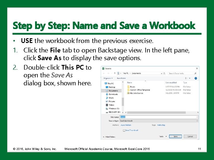
Step by Step: Name and Save a Workbook • USE the workbook from the previous exercise. 1. Click the File tab to open Backstage view. In the left pane, click Save As to display the save options. 2. Double-click This PC to open the Save As dialog box, shown here. © 2016, John Wiley & Sons, Inc. Microsoft Official Academic Course, Microsoft Excel Core 2016 11

Step by Step: Name and Save a Workbook 3. In the navigation pane on the left, in the Save As dialog box, click Desktop. The Desktop becomes the new destination of your saved file. 4. In the Save As dialog box, click New folder. A folder icon appears with the words New folder selected. 5. Type Excel Lesson 2 and then press Enter. 6. Click the Open button. 7. In the File name box, type 02 Fabrikam Address Solution. 8. Click the Save button. • LEAVE the workbook open to use in the next exercise. © 2016, John Wiley & Sons, Inc. Microsoft Official Academic Course, Microsoft Excel Core 2016 12

Saving to Your One. Drive • One. Drive is a cloud-based application that allows you to store and sync your files so you can retrieve them anywhere and share them. • One. Drive is a great place to store backup files of important documents. • One. Drive comes with recent versions of Windows and Microsoft Office. • A free desktop app is available for mobile devices. © 2016, John Wiley & Sons, Inc. Microsoft Official Academic Course, Microsoft Excel Core 2016 13

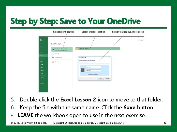
Step by Step: Save to Your One. Drive • USE the workbook from the previous exercise. 1. Click the File tab and then click Save As. 2. In the Backstage view, under Save As, click your One. Drive account, and then click a folder location in the right pane. You may need to sign in to One. Drive if you haven’t already (see the figure on the next slide). 3. Click the New folder button in the Save As dialog box. 4. In the New folder text box, type Excel Lesson 2 to save a folder for this lesson on your One. Drive and then press Enter. © 2016, John Wiley & Sons, Inc. Microsoft Official Academic Course, Microsoft Excel Core 2016 14

Step by Step: Save to Your One. Drive 5. Double-click the Excel Lesson 2 icon to move to that folder. 6. Keep the file with the same name. Click the Save button. • LEAVE the workbook open to use in the next exercise. © 2016, John Wiley & Sons, Inc. Microsoft Official Academic Course, Microsoft Excel Core 2016 15

Step by Step: Save a Workbook Under a Different Name • 1. 2. 3. USE the workbook from the previous exercise. In cell A 2, type 87 East Broad Street and then press Enter. In cell A 3, type Columbus, OH 43215 and then press Enter. Click the File tab, and in the left pane, click Save As. The Backstage view shows that the Current Folder in the right pane is Excel Lesson 2 on your One. Drive, because it was the folder that was last used to save a workbook. 4. Click This PC to return to the drive you used before. 5. In the right pane, click Excel Lesson 2. 6. Click in the File name box, click after Fabrikam, and then type Broad so the name reads 02 Fabrikam Broad Address Solution. © 2016, John Wiley & Sons, Inc. Microsoft Official Academic Course, Microsoft Excel Core 2016 16

Step by Step: Save a Workbook Under a Different Name 7. Click Save. You created a new workbook by saving an existing workbook with a new name. 8. Click the File tab, click Save As in the left pane, and then click Browse. 9. In the File name box, type 02 Fabrikam Broad Address Template Solution. 10. In the Save as type box, click the drop-down arrow and then choose Excel Template. Click the Save button. • CLOSE Excel. © 2016, John Wiley & Sons, Inc. Microsoft Official Academic Course, Microsoft Excel Core 2016 17

Saving a Workbook in a Previous Excel Format • Files created in earlier Excel versions can be opened and revised in Excel 2016. • Users who use earlier versions of Excel or other applications, might not be able to open your file. • You can save a copy of an Excel 2016 workbook (with the. xlsx file extension) to the older Excel 97 -2003 Workbook format (with the. xls file extension). • The program symbol displayed with the filenames is different, but give the earlier edition a different name. • Check which features might be lost with Excel’s compatibility checker. © 2016, John Wiley & Sons, Inc. Microsoft Official Academic Course, Microsoft Excel Core 2016 18

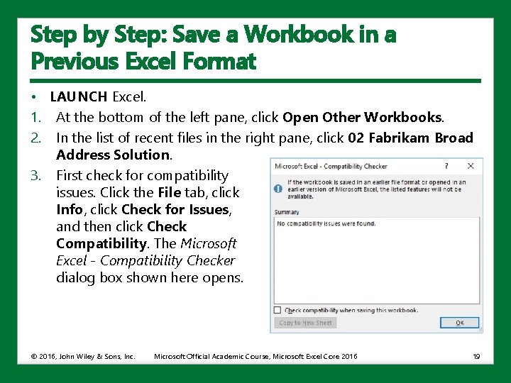
Step by Step: Save a Workbook in a Previous Excel Format • LAUNCH Excel. 1. At the bottom of the left pane, click Open Other Workbooks. 2. In the list of recent files in the right pane, click 02 Fabrikam Broad Address Solution. 3. First check for compatibility issues. Click the File tab, click Info, click Check for Issues, and then click Check Compatibility. The Microsoft Excel - Compatibility Checker dialog box shown here opens. © 2016, John Wiley & Sons, Inc. Microsoft Official Academic Course, Microsoft Excel Core 2016 19

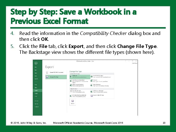
Step by Step: Save a Workbook in a Previous Excel Format 4. 5. Read the information in the Compatibility Checker dialog box and then click OK. Click the File tab, click Export, and then click Change File Type. The Backstage view shows the different file types (shown here). © 2016, John Wiley & Sons, Inc. Microsoft Official Academic Course, Microsoft Excel Core 2016 20

Step by Step: Save a Workbook in a Previous Excel Format 6. Click Excel 97 -2003 Workbook and then click Save As. 7. In the File name box, click before Solution, type 97 -03, and then click Save. 8. Click the File tab, and then click Close to close the 02 Fabrikam Broad Address 97 -03 Solution workbook. 9. Click the File tab and then click Open. The right pane in Backstage view shows the last set of documents that have been saved. 10. Click 02 Fabrikam Broad Address Solution. • LEAVE the workbook open to use in the next exercise. © 2016, John Wiley & Sons, Inc. Microsoft Official Academic Course, Microsoft Excel Core 2016 21

Saving in Different File Formats • You can save an Excel 2016 file in a format other than. xlsx or. xls. • The file formats listed as options in the Save As dialog box or on the Export tab depend on what type of file format the application supports. • When you save a file in another file format, some of the formatting, data, and features might be lost. © 2016, John Wiley & Sons, Inc. Microsoft Official Academic Course, Microsoft Excel Core 2016 22

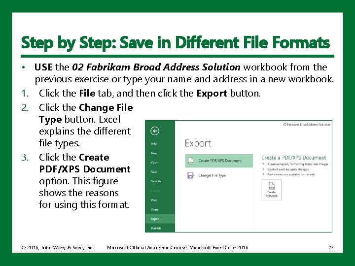
Step by Step: Save in Different File Formats • USE the 02 Fabrikam Broad Address Solution workbook from the previous exercise or type your name and address in a new workbook. 1. Click the File tab, and then click the Export button. 2. Click the Change File Type button. Excel explains the different file types. 3. Click the Create PDF/XPS Document option. This figure shows the reasons for using this format. © 2016, John Wiley & Sons, Inc. Microsoft Official Academic Course, Microsoft Excel Core 2016 23

Step by Step: Save in Different File Formats 4. 5. 6. 7. In the right pane, click the Create PDF/XPS button. In the left navigation pane, click Desktop. Double-click Excel Lesson 2 to move to that folder. In the Publish as PDF or XPS dialog box, ensure that the Save as type list shows PDF. 8. Click Publish. 9. The Reader application (or a Web browser) opens with the PDF file displayed. 10. Press Alt+F 4 to close the browser or Reader application. 11. If necessary, press Alt+Tab to return to the Excel file. • CLOSE the workbook and LEAVE Excel open to use in the next exercise. © 2016, John Wiley & Sons, Inc. Microsoft Official Academic Course, Microsoft Excel Core 2016 24

Entering and Editing Basic Data in a Worksheet • You can type data directly into a worksheet cell. • You can also copy and paste information from another worksheet or from other programs. • Copy takes the information from one location and duplicates it. • Paste puts this information into another location. • To enter data in a cell in a worksheet, the cell must be active then you the data. To move to the next column, press Tab. • When you finish typing the entries in a row, press Enter to move to the beginning of the next row. • Use the arrow keys to move to an adjacent cell or click on any cell to make that cell active. • Press Enter to accept the entry and move down one row. © 2016, John Wiley & Sons, Inc. Microsoft Official Academic Course, Microsoft Excel Core 2016 25

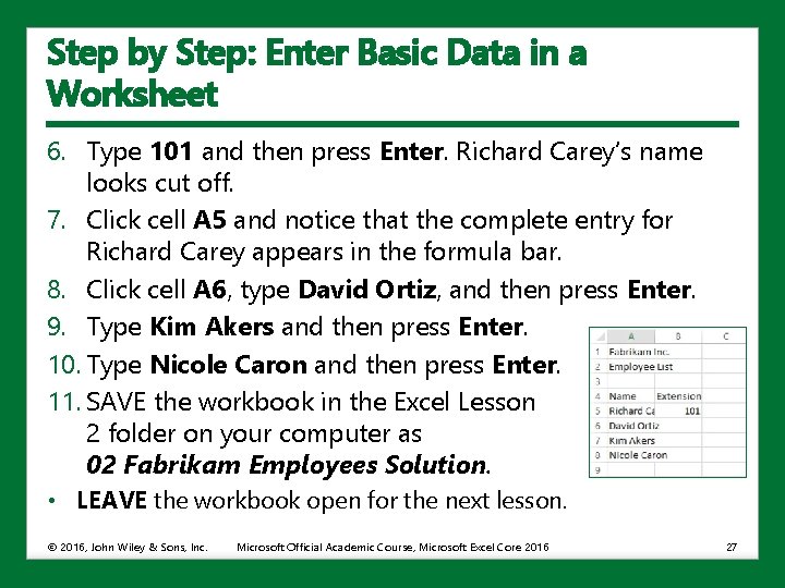
Step by Step: Enter Basic Data in a Worksheet • If necessary LAUNCH Excel and OPEN a new workbook. 1. Click cell A 1, type Fabrikam Inc. , and then press Enter. Notice that the active cell moves to the next row, to cell A 2. 2. In cell A 2, type Employee List and then press Enter. 3. Click cell A 4, type Name, and then press Tab. Notice that the active cell moves to the next column, to cell B 4. 4. Type Extension and then press Enter. Notice that the active cell moves to the first cell in the next row. 5. Type Richard Carey and then press Tab. © 2016, John Wiley & Sons, Inc. Microsoft Official Academic Course, Microsoft Excel Core 2016 26

Step by Step: Enter Basic Data in a Worksheet 6. Type 101 and then press Enter. Richard Carey’s name looks cut off. 7. Click cell A 5 and notice that the complete entry for Richard Carey appears in the formula bar. 8. Click cell A 6, type David Ortiz, and then press Enter. 9. Type Kim Akers and then press Enter. 10. Type Nicole Caron and then press Enter. 11. SAVE the workbook in the Excel Lesson 2 folder on your computer as 02 Fabrikam Employees Solution. • LEAVE the workbook open for the next lesson. © 2016, John Wiley & Sons, Inc. Microsoft Official Academic Course, Microsoft Excel Core 2016 27

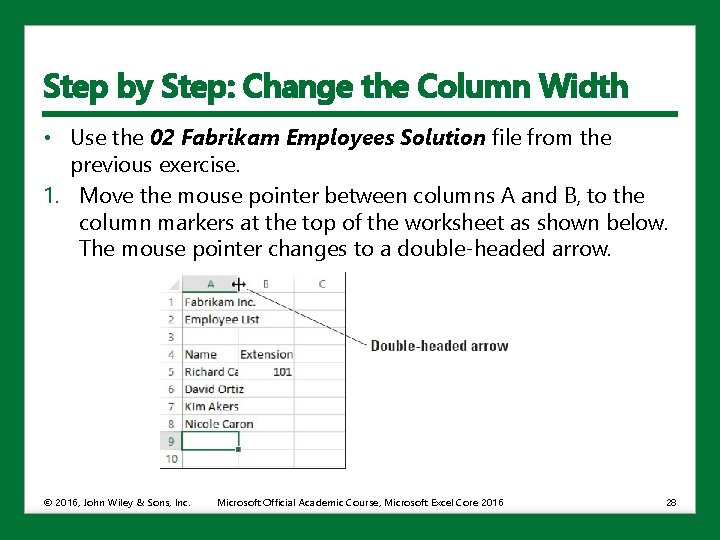
Step by Step: Change the Column Width • Use the 02 Fabrikam Employees Solution file from the previous exercise. 1. Move the mouse pointer between columns A and B, to the column markers at the top of the worksheet as shown below. The mouse pointer changes to a double-headed arrow. © 2016, John Wiley & Sons, Inc. Microsoft Official Academic Course, Microsoft Excel Core 2016 28

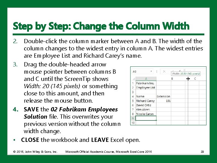
Step by Step: Change the Column Width 2. Double-click the column marker between A and B. The width of the column changes to the widest entry in column A. The widest entries are Employee List and Richard Carey’s name. 3. Drag the double-headed arrow mouse pointer between columns B and C until the Screen. Tip shows Width: 20 (145 pixels) or something close to this amount, and then release the mouse button. 4. SAVE the 02 Fabrikam Employees Solution file. This overwrites your previous version without the column width change. • CLOSE the workbook and LEAVE Excel open. © 2016, John Wiley & Sons, Inc. Microsoft Official Academic Course, Microsoft Excel Core 2016 29

Editing a Cell’s Contents • Changes can be made quickly and easily in electronic records. • To edit information in a worksheet, make changes directly in the cell or edit the contents of a cell in the formula bar. • When you enter data in a cell, the text or numbers appear in the cell and in the formula bar. • Before changes can be made, you must select the information that is to be changed. • Selecting text means that you highlight the text to be changed. • You can select a single cell or a portion of the cell’s text in the formula bar. • You can also double-click in a cell to position the insertion point for editing. © 2016, John Wiley & Sons, Inc. Microsoft Official Academic Course, Microsoft Excel Core 2016 30

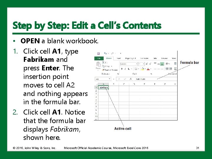
Step by Step: Edit a Cell’s Contents • OPEN a blank workbook. 1. Click cell A 1, type Fabrikam and press Enter. The insertion point moves to cell A 2 and nothing appears in the formula bar. 2. Click cell A 1. Notice that the formula bar displays Fabrikam, shown here. © 2016, John Wiley & Sons, Inc. Microsoft Official Academic Course, Microsoft Excel Core 2016 31

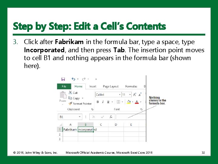
Step by Step: Edit a Cell’s Contents 3. Click after Fabrikam in the formula bar, type a space, type Incorporated, and then press Tab. The insertion point moves to cell B 1 and nothing appears in the formula bar (shown here). © 2016, John Wiley & Sons, Inc. Microsoft Official Academic Course, Microsoft Excel Core 2016 32

Step by Step: Edit a Cell’s Contents 4. Click cell A 1 and in the formula bar, double-click on Incorporated to select it. Type Inc. and then press Enter. 5. Type Sales and then press Enter. 6. Click cell A 2 and then click after Sales in the formula bar. 7. Press Home. The insertion point moves to the beginning of the formula bar. 8. Type Monthly and then press the spacebar. Press Enter. 9. In cell A 3, type January and then press Enter. © 2016, John Wiley & Sons, Inc. Microsoft Official Academic Course, Microsoft Excel Core 2016 33

Step by Step: Edit a Cell’s Contents 10. Click cell A 3, type February, and then press Enter. Cell A 3’s original text is gone and February replaces January. 11. Click cell A 3 and then press Delete. The entry in A 3 is removed. 12. Above row 1 and to the left of column A, click the Select All button. All cells on the worksheet are selected. 13. Press Delete. All entries are removed. • CLOSE the workbook without saving and LEAVE Excel open for the next exercise. © 2016, John Wiley & Sons, Inc. Microsoft Official Academic Course, Microsoft Excel Core 2016 34

Step by Step: Edit a Cell’s Contents • When you are in Edit mode: • The insertion point appears as a vertical bar and most commands are inactive. • You can move the insertion point by using the left and right arrow keys. • The Edit indicator appears at the left end of the Status bar. • Use the Home key on your keyboard to move the insertion point to the beginning of the cell, and use the End key to move the insertion point to the end of the cell. • You can add new characters at the location of the insertion point. © 2016, John Wiley & Sons, Inc. Microsoft Official Academic Course, Microsoft Excel Core 2016 35

Step by Step: Edit a Cell’s Contents • To select multiple characters while in Edit mode, press Shift while you press the arrow keys. • You also can use the to click and drag the mouse pointer over the characters that you want to select. • There are several ways to modify the values or text you enter into a cell: • Erase the cell’s contents. • Replace the cell’s contents with something else. • Edit the cell’s contents. © 2016, John Wiley & Sons, Inc. Microsoft Official Academic Course, Microsoft Excel Core 2016 36

Deleting and Clearing a Cell’s Contents • To erase the what’s in a cell rather than the cell itself, click the cell and then press Delete. • To erase the contents of more than one cell, select all the cells that you want to erase and on your keyboard, press Delete. • Pressing Delete removes the cell’s contents, but does not remove any formatting. © 2016, John Wiley & Sons, Inc. Microsoft Official Academic Course, Microsoft Excel Core 2016 37

Step by Step: Delete and Clear a Cell’s Contents • 1. 2. 3. 4. 5. OPEN a blank workbook. In cell A 1, type 1 and then press Enter. Type 2 and then press Enter. Type 3 and then press Enter. Type 4 and then press Enter. Highlight cells A 1 through A 4 (containing the numbers 1 through 4). 6. Press Delete. All the cells are erased. 7. On the Quick Access Toolbar, click the Undo button to restore the cell entries. 8. Click cell B 5, type $275, 000, and then press Enter. The value and format are placed into the cell. © 2016, John Wiley & Sons, Inc. Microsoft Official Academic Course, Microsoft Excel Core 2016 38

Step by Step: Delete and Clear a Cell’s Contents 9. Click cell B 5 and then press Delete. 10. Type 225000 without the dollar sign and comma and then press Enter. Notice that $225, 000 is formatted. Although the original entry is gone, the cell retains the previous format when you press Delete. 11. Click cell B 5 and on the Home tab, in the Editing group, click Clear. 12. Click Clear Formats. Cell B 5 displays 225000 without the dollar sign and comma. • CLOSE the workbook without saving and LEAVE Excel open for the next exercise. © 2016, John Wiley & Sons, Inc. Microsoft Official Academic Course, Microsoft Excel Core 2016 39

Using Data Types to Populate a Worksheet • You can enter three types of data into Excel: text, numbers, and formulas. • Text entries contain alphabetic characters and any other characters that do not have a purely numeric value. • The strength of Excel is its capability to calculate and analyze numbers based on the numeric values you enter. Of course, if you enter the wrong numbers, you get the wrong calculations. For that reason, accurate data entry is crucial. © 2016, John Wiley & Sons, Inc. Microsoft Official Academic Course, Microsoft Excel Core 2016 40

Entering Dates • Dates are often used in worksheets to track data over a specified period of time. • Dates can be used as row and column headings. • Dates are serial numbers. They are sequential and can be added, subtracted, and used in calculations. • Dates can also be used in formulas and in developing graphs and charts. • The way a date is displayed in a worksheet cell depends on the format in which you type the characters. • In Excel 2016, the default date format uses four digits for the year and the date is right-justified. © 2016, John Wiley & Sons, Inc. Microsoft Official Academic Course, Microsoft Excel Core 2016 41

Step by Step: Enter Dates • OPEN 02 Fabrikam Sales from the data files for this lesson. 1. Click cell B 5, type 1/4/2017, and then press Enter. 2. Click cell B 6, type 1/25/17, and then press Enter. The date is entered and B 7 becomes the active cell. 3. Type 1/23 and then press Enter. 23 -Jan is entered in the cell. Click cell B 7, and notice that 1/23/20 XX (with XX representing the current year) appears in the formula bar. 4. If the year displayed in the formula bar is not 2017, click cell B 7 and then press F 2. Change the year to 2017 and then press Enter. 5. In cell B 8, type 1/28/17 and then press Enter. © 2016, John Wiley & Sons, Inc. Microsoft Official Academic Course, Microsoft Excel Core 2016 42

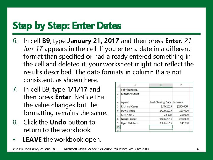
Step by Step: Enter Dates 6. In cell B 9, type January 21, 2017 and then press Enter. 21 Jan-17 appears in the cell. If you enter a date in a different format than specified or had already entered something in the cell and deleted it, your worksheet might not reflect the results described. The date formats in column B are not consistent, as shown here. 7. In cell B 9, type 1/1/17 and then press Enter. Notice that the value changes but the formatting remains the same. 8. Click the Undo button to return to the workbook. • LEAVE the workbook open. © 2016, John Wiley & Sons, Inc. Microsoft Official Academic Course, Microsoft Excel Core 2016 43

Step by Step: Enter Dates • Excel interprets two-digit years from 00 to 29 as the years 2000 to 2029. • Two-digit years from 30 to 99 are interpreted as 1930 to 1999. • If you type January 28, 2020, the date will display as 28 -Jan-20. • If you type 1/28 without a year, Excel interprets the date to be the current year. • The formula bar always displays the date in month/day/fourdigit-year format because that is the format required for calculations and analyses. © 2016, John Wiley & Sons, Inc. Microsoft Official Academic Course, Microsoft Excel Core 2016 44

Filling a Series with Auto Fill • Excel provides Auto Fill options that automatically fill cells with data and/or formatting. • To populate a new cell with data that exists in an adjacent cell, use the Auto Fill feature either through the command or the fill handle. • The fill handle is a small green square in the lower-right corner of a selected cell or range of cells. • A range is a group of adjacent cells that you select to perform operations on all of the selected cells. • When you refer to a range of cells, the first cell and last cell are separated by a colon (for example, C 4: H 4). © 2016, John Wiley & Sons, Inc. Microsoft Official Academic Course, Microsoft Excel Core 2016 45

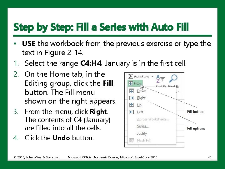
Step by Step: Fill a Series with Auto Fill • USE the workbook from the previous exercise or type the text in Figure 2 -14. 1. Select the range C 4: H 4. January is in the first cell. 2. On the Home tab, in the Editing group, click the Fill button. The Fill menu shown on the right appears. 3. From the menu, click Right. The contents of C 4 (January) are filled into all the cells. 4. Click the Undo button. © 2016, John Wiley & Sons, Inc. Microsoft Official Academic Course, Microsoft Excel Core 2016 46

Step by Step: Fill a Series with Auto Fill 5. Select the range C 9: C 13 and then click the Fill button. Choose Down to copy C 9 into the four additional cells. 6. Click the Undo button. 7. Click cell C 4, point to the fill handle in the lower-right corner of the cell (see below), and drag it to E 4 and release. The Auto Fill Options button appears next to the range, and January through March are displayed. © 2016, John Wiley & Sons, Inc. Microsoft Official Academic Course, Microsoft Excel Core 2016 47

Step by Step: Fill a Series with Auto Fill 8. Click cell C 5, point to the fill handle, and then drag it to C 9 and release. All the numbers turn to $275, 000 in column C. The Auto Fill Options button appears near the lower-right corner of the selected range (see below). 9. Click the Auto Fill Options button, and choose Fill Formatting Only from the list that appears. The numbers return to their previous values with new formatting. © 2016, John Wiley & Sons, Inc. Microsoft Official Academic Course, Microsoft Excel Core 2016 48

Step by Step: Fill a Series with Auto Fill 10. Repeat Steps 8 and 9 for the range B 5: B 9. 11. Click cell A 9, and then drag the fill handle down to A 15. Ryan Calafato’s name is repeated. 12. Click the Undo button to return the spreadsheet. 13. SAVE the workbook as 02 Fabrikam Sales Solution. • CLOSE the workbook and LEAVE Excel open for the next exercise. © 2016, John Wiley & Sons, Inc. Microsoft Official Academic Course, Microsoft Excel Core 2016 49

Step by Step: Fill a Series with Auto Fill • After you fill cells using the fill handle, the Auto Fill Options button appears so that you can choose how the selection is filled. • In Excel, the default option is to copy the original content and formatting. • With Auto Fill, you can select how the content of the original cell appears in each cell in the filled range. • A natural series is a formatted series of text or numbers that are in a normal sequence such as months, weekdays, numbers, or times. • The table on the next slide shows different natural series that Excel automatically recognizes. © 2016, John Wiley & Sons, Inc. Microsoft Official Academic Course, Microsoft Excel Core 2016 50

Step by Step: Fill a Series with Auto Fill © 2016, John Wiley & Sons, Inc. Microsoft Official Academic Course, Microsoft Excel Core 2016 51

Filling a Series with Flash Fill • Flash Fill allows you to quickly fill a column of data using an example that is based on existing data in adjacent columns. • You can almost instantly create columns for first and last names if the full name appears in another column. • After you enter the initial item (such as the first name) in a column and start to type the second item in that column, Excel displays a preview of entries formatted the same way in the rest of the column. • If the presented preview of the data is what you want, just press Enter to fill the column with the entries. © 2016, John Wiley & Sons, Inc. Microsoft Official Academic Course, Microsoft Excel Core 2016 52

Step by Step: Fill a Series with Flash Fill • OPEN 02 Customers from the data files for this lesson. 1. Notice the customer list in column A, which includes the last name followed by a comma and then the first name. You want to create separate columns for the first and last names. 2. Select cell B 2 in the First Name column. 3. Type Alice and then press Enter. 4. In cell B 3, type Ai to begin the next first name, Aidan. Excel guesses that you want to enter the rest of the first names in column B and displays a preview of the results (shown on the next slide). © 2016, John Wiley & Sons, Inc. Microsoft Official Academic Course, Microsoft Excel Core 2016 53

Step by Step: Fill a Series with Flash Fill 5. Press Enter to accept the suggestion. The remaining first names fill down the column. Excel also includes the middle initials for those names that include them. © 2016, John Wiley & Sons, Inc. Microsoft Official Academic Course, Microsoft Excel Core 2016 54

Step by Step: Fill a Series with Flash Fill 6. Select cell C 2 in the Last Name column. 7. Type Ciccu and then press Enter. 8. In cell C 3, type De to begin the next last name, Delaney. Excel guesses that you want to enter the rest of the last names in column C and displays a preview of the results. 9. Press Enter to accept the suggestion. The remaining last names fill down the column. 10. SAVE the workbook as 02 Customers Solution. • CLOSE Excel. © 2016, John Wiley & Sons, Inc. Microsoft Official Academic Course, Microsoft Excel Core 2016 55

Cutting, Copying, and Pasting Data • Excel’s Cut, Copy, and Paste commands are used to copy or move entire cells with their contents, formats, and formulas. • You can copy specific contents or attributes from the cells. • You can copy the value from the original cell but retain the formatting of the destination cell. • You can perform cut, copy, and paste functions using: • The mouse • Ribbon commands • Shortcut commands, such as Ctrl+C (copy), Ctrl+X (cut), and Ctrl+V (paste) • The Office Clipboard pane © 2016, John Wiley & Sons, Inc. Microsoft Official Academic Course, Microsoft Excel Core 2016 56

Copying a Data Series with the Mouse • By default, drag-and-drop editing is turned on so that you can use the mouse to copy (duplicate) or move cells. • Select the cell or range of cells you want to copy and hold down Ctrl while you point to the border of the selection. • When the pointer becomes a copy pointer (arrow with a plus), you can drag the cell or range of cells to the new location. • As you drag, a scrolling Screen. Tip identifies where the selection will be copied if you release the mouse button. © 2016, John Wiley & Sons, Inc. Microsoft Official Academic Course, Microsoft Excel Core 2016 57

Step by Step: Copy a Data Series with the Mouse • Before you begin these steps, LAUNCH Microsoft Excel. 1. 2. 3. Open the 02 Customer Houses file. Select the range A 12: A 22. Press Ctrl and point to the right border of the selected range. The copy pointer is displayed. 4. With the copy pointer displayed, press and hold down the left mouse button and drag the selection to the right, until H 12: H 22 appears in the scrolling Screen. Tip next to the selection. 5. Release the mouse button and then release Ctrl. The data in A 12: A 22 also appears in H 12: H 22. • LEAVE the workbook open to use in the next exercise. © 2016, John Wiley & Sons, Inc. Microsoft Official Academic Course, Microsoft Excel Core 2016 58

Moving a Data Series with the Mouse • Data can be moved from one location to another within a workbook in much the same way as copying. • To move a data series, select the cell or range of cells and point to the border of the selection. • When the pointer becomes a move pointer, you can drag the cell or range of cells to a new location. • When data is moved, it replaces any existing data in the destination cells. © 2016, John Wiley & Sons, Inc. Microsoft Official Academic Course, Microsoft Excel Core 2016 59

Step by Step: Move a Data Series with the Mouse • USE the 02 Customer Houses workbook from the previous exercise. 1. Select E 12: E 22. 2. Point to the right border of the selected range. The move pointer (a white arrow with four smaller black arrows attached) is displayed. 3. With the move pointer displayed, hold down the left mouse button and then drag the selection to the right, until I 12: I 22 appears in the scrolling Screen. Tip beside the selected range. 4. Release the mouse button. In your worksheet, the destination cells are empty; therefore, you are not concerned with replacing existing data. The data previously in E 12: E 22 is now in I 12: I 22. © 2016, John Wiley & Sons, Inc. Microsoft Official Academic Course, Microsoft Excel Core 2016 60

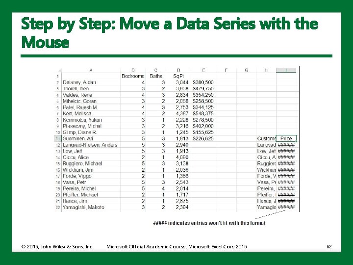
Step by Step: Move a Data Series with the Mouse 1. Drag A 1 to H 12. Note that a dialog box warns you about replacing the contents of the destination cells. 2. Click Cancel. 3. Drag A 1 to H 11. 4. Drag E 1 to I 11. Your worksheet should look like the one shown on the next slide. • LEAVE the workbook open to use in the next exercise. © 2016, John Wiley & Sons, Inc. Microsoft Official Academic Course, Microsoft Excel Core 2016 61

Step by Step: Move a Data Series with the Mouse © 2016, John Wiley & Sons, Inc. Microsoft Official Academic Course, Microsoft Excel Core 2016 62

Copying and Pasting Data • The Office Clipboard collects and stores up to 24 copied or cut items that are then available to be used in Excel and in other Microsoft Office programs. • You can paste (insert) selected items from the Clipboard to a new location in the worksheet. • Cut (moved) data is removed from the worksheet but is still available for you to use in multiple locations. • If you copy multiple items and then click Paste, only the last item copied will be pasted. • To access multiple items, you must open the Clipboard pane. © 2016, John Wiley & Sons, Inc. Microsoft Official Academic Course, Microsoft Excel Core 2016 63

Step by Step: Copy and Paste Data • USE the 02 Customer Houses workbook from the previous exercise. 1. On the Home tab of the ribbon, click the Clipboard Dialog Box Launcher. The Clipboard pane opens on the left side of the worksheet. 2. Select A 1: E 22 and then press Delete. 3. Select H 11: I 22 and in the Clipboard group, click the Copy button. The border around the selected range becomes a moving border. 4. Select A 1 and then click the Paste button. The moving border remains active around H 11: I 22. A copied range does not deactivate until you type new text, issue another command, double-click on another cell, or press Esc. © 2016, John Wiley & Sons, Inc. Microsoft Official Academic Course, Microsoft Excel Core 2016 64

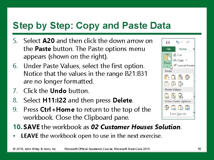
Step by Step: Copy and Paste Data 5. Select A 20 and then click the down arrow on the Paste button. The Paste options menu appears (shown on the right). 6. Under Paste Values, select the first option. Notice that the values in the range B 21: B 31 are no longer formatted. 7. Click the Undo button. 8. Select H 11: I 22 and then press Delete. 9. Press Ctrl+Home to return to the top of the workbook. Close the Clipboard pane. 10. SAVE the workbook as 02 Customer Houses Solution. • LEAVE the workbook open to use in the next exercise. © 2016, John Wiley & Sons, Inc. Microsoft Official Academic Course, Microsoft Excel Core 2016 65

Editing a Workbook’s Properties • The workbook has a number of properties that are associated with it to make managing it easier. • The properties include items that you indirectly change such as file size and last edit date. • The workbook properties also include items you directly change such as keywords. • Assigning keywords (also called tags) to the document properties makes it easier to organize and find documents. • You can also add more notes to your file for classification and document management. © 2016, John Wiley & Sons, Inc. Microsoft Official Academic Course, Microsoft Excel Core 2016 66

Step by Step: Assign Keywords • USE the 02 Customer Houses Solution workbook from the previous exercise. 1. Click File. The Backstage view displays current properties on the right side of the window. 2. At the bottom of the right pane, click the Show All Properties link to display additional properties. 3. Click the Tags field and type Customer, Sq Ft, Price. 4. Click the Categories field and type Revenue. 5. Click the Company field and type Fabrikam, Inc. . © 2016, John Wiley & Sons, Inc. Microsoft Official Academic Course, Microsoft Excel Core 2016 67

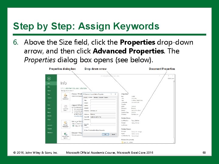
Step by Step: Assign Keywords 6. Above the Size field, click the Properties drop-down arrow, and then click Advanced Properties. The Properties dialog box opens (see below). © 2016, John Wiley & Sons, Inc. Microsoft Official Academic Course, Microsoft Excel Core 2016 68

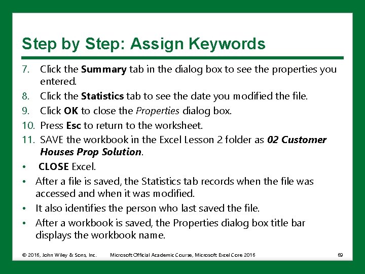
Step by Step: Assign Keywords 7. Click the Summary tab in the dialog box to see the properties you entered. 8. Click the Statistics tab to see the date you modified the file. 9. Click OK to close the Properties dialog box. 10. Press Esc to return to the worksheet. 11. SAVE the workbook in the Excel Lesson 2 folder as 02 Customer Houses Prop Solution. • CLOSE Excel. • After a file is saved, the Statistics tab records when the file was accessed and when it was modified. • It also identifies the person who last saved the file. • After a workbook is saved, the Properties dialog box title bar displays the workbook name. © 2016, John Wiley & Sons, Inc. Microsoft Official Academic Course, Microsoft Excel Core 2016 69

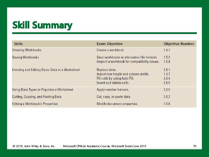
Skill Summary © 2016, John Wiley & Sons, Inc. Microsoft Official Academic Course, Microsoft Excel Core 2016 70