Microsoft Excel 2013 Lesson 8 Managing Worksheets 2014

Microsoft Excel 2013 Lesson 8 Managing Worksheets © 2014, John Wiley & Sons, Inc. Microsoft Official Academic Course, Microsoft Word 2013 1

Objectives © 2014, John Wiley & Sons, Inc. Microsoft Official Academic Course, Microsoft Word 2013 2

Software Orientation • In this lesson, you become familiar with how a workbook contains worksheets, and how you manipulate those worksheets within a workbook the way you might reorganize the contents of a folder in your desk drawer. • Unlike the old desk drawer, though, you have a few tools that will remind you that you’re using a computer, such as the Find command to help you search for certain contents. © 2014, John Wiley & Sons, Inc. Microsoft Official Academic Course, Microsoft Word 2013 3

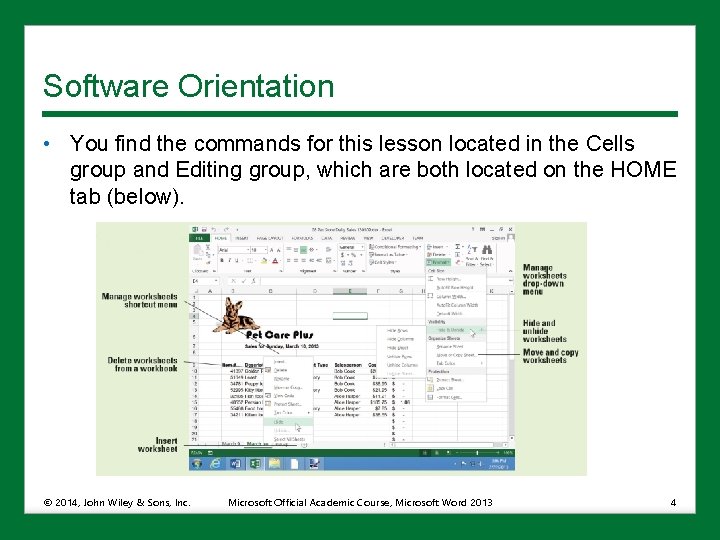
Software Orientation • You find the commands for this lesson located in the Cells group and Editing group, which are both located on the HOME tab (below). © 2014, John Wiley & Sons, Inc. Microsoft Official Academic Course, Microsoft Word 2013 4

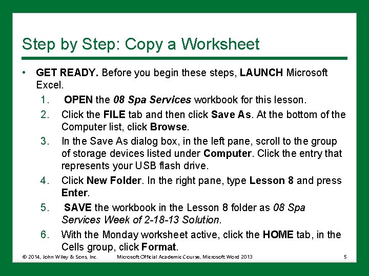
Step by Step: Copy a Worksheet • GET READY. Before you begin these steps, LAUNCH Microsoft Excel. 1. OPEN the 08 Spa Services workbook for this lesson. 2. Click the FILE tab and then click Save As. At the bottom of the Computer list, click Browse. 3. In the Save As dialog box, in the left pane, scroll to the group of storage devices listed under Computer. Click the entry that represents your USB flash drive. 4. Click New Folder. In the right pane, type Lesson 8 and press Enter. 5. SAVE the workbook in the Lesson 8 folder as 08 Spa Services Week of 2 -18 -13 Solution. 6. With the Monday worksheet active, click the HOME tab, in the Cells group, click Format. © 2014, John Wiley & Sons, Inc. Microsoft Official Academic Course, Microsoft Word 2013 5

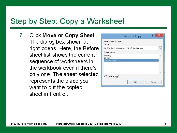
Step by Step: Copy a Worksheet 7. Click Move or Copy Sheet. The dialog box shown at right opens. Here, the Before sheet list shows the current sequence of worksheets in the workbook even if there’s only one. The sheet selected represents the place you want to put the copied sheet in front of. © 2014, John Wiley & Sons, Inc. Microsoft Official Academic Course, Microsoft Word 2013 6

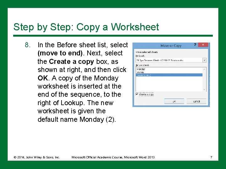
Step by Step: Copy a Worksheet 8. In the Before sheet list, select (move to end). Next, select the Create a copy box, as shown at right, and then click OK. A copy of the Monday worksheet is inserted at the end of the sequence, to the right of Lookup. The new worksheet is given the default name Monday (2). © 2014, John Wiley & Sons, Inc. Microsoft Official Academic Course, Microsoft Word 2013 7

Step by Step: Copy a Worksheet 9. Click the Monday worksheet tab. Next, click and hold the Monday tab, and then press and hold Ctrl. The pointer changes from an arrow to a paper with a plus sign in it. 10. Drag the pointer to the right until the down-arrow just above the tabs bar points to the divider to the right of Monday (2). Release the mouse button and Ctrl key. A new worksheet is created, with its tab located just to the right of where the down-arrow was pointing. Its name is Monday (3). 11. With Monday (3) active, click cell B 4 and type the date 2/19/2013. © 2014, John Wiley & Sons, Inc. Microsoft Official Academic Course, Microsoft Word 2013 8

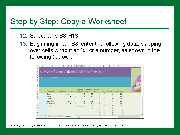
Step by Step: Copy a Worksheet 12. Select cells B 8: H 13. Beginning in cell B 8, enter the following data, skipping over cells without an “x” or a number, as shown in the following (below): © 2014, John Wiley & Sons, Inc. Microsoft Official Academic Course, Microsoft Word 2013 9

Step by Step: Copy a Worksheet • PAUSE. SAVE the workbook and LEAVE it open to use in the next exercise. © 2014, John Wiley & Sons, Inc. Microsoft Official Academic Course, Microsoft Word 2013 10

Step by Step: Rename a Worksheet • GET READY. USE the workbook from the previous exercise. 1. Double-click the Monday (3) worksheet tab to select its name. 2. Type Tuesday and press Enter. The new name appears on the tab. 3. Repeat this process for the Monday (2) worksheet tab, renaming it Wednesday. 4. With the Wednesday worksheet active, select cell B 4 and type the date 2/20/2013. 5. Select cells B 8: H 15. © 2014, John Wiley & Sons, Inc. Microsoft Official Academic Course, Microsoft Word 2013 11

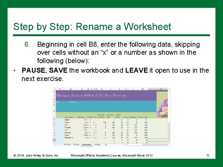
Step by Step: Rename a Worksheet 6. Beginning in cell B 8, enter the following data, skipping over cells without an “x” or a number as shown in the following (below): • PAUSE. SAVE the workbook and LEAVE it open to use in the next exercise. © 2014, John Wiley & Sons, Inc. Microsoft Official Academic Course, Microsoft Word 2013 12

Step by Step: Reposition the Worksheets in a Workbook • GET READY. USE the workbook from the previous exercise. 1. Click the Tuesday worksheet tab. On the HOME tab, in the Cells group, click Format. 2. Click Move or Copy Sheet. The Move or Copy dialog box opens. 3. To make sure Tuesday appears before Wednesday, click Wednesday in the Before sheet list, and then click OK. © 2014, John Wiley & Sons, Inc. Microsoft Official Academic Course, Microsoft Word 2013 13

Step by Step: Reposition the Worksheets in a Workbook 1. Click and hold the Lookup worksheet tab. The pointer changes from an arrow to a paper without a plus sign. 2. Drag the pointer to the right until the down-arrow just above the tabs bar points to the divider to the right of Wednesday. Release the mouse button. The Lookup worksheet is repositioned at the end of the sequence, and nothing inside the worksheet itself is changed. 3. Click the Monday worksheet tab. © 2014, John Wiley & Sons, Inc. Microsoft Official Academic Course, Microsoft Word 2013 14

Step by Step: Reposition the Worksheets in a Workbook 4. Select cells B 8: H 11. 5. Beginning in cell B 8, enter the following data, skipping over cells without an “x” or a number as shown in the following: • PAUSE. SAVE the workbook and LEAVE it open to use in the next exercise. © 2014, John Wiley & Sons, Inc. Microsoft Official Academic Course, Microsoft Word 2013 15

Step by Step: Change the Color of a Worksheet Tab • GET READY. USE the workbook from the previous exercise. 1. Right-click the Monday worksheet tab. 2. In the shortcut menu, click Tab Color. 3. In the popup menu, under Standard Colors, click Red. Excel gives a slightly red tint to the Monday worksheet tab. 4. Click the Tuesday worksheet tab. Notice the Monday worksheet tab is now the bold red color you chose. Excel applies only the gradient tint to the tab for the currently visible worksheet to make it stand out above the others. 5. Repeat the color selection process for the Tuesday and Wednesday worksheet tabs, choosing Orange and Yellow, respectively. © 2014, John Wiley & Sons, Inc. Microsoft Official Academic Course, Microsoft Word 2013 16

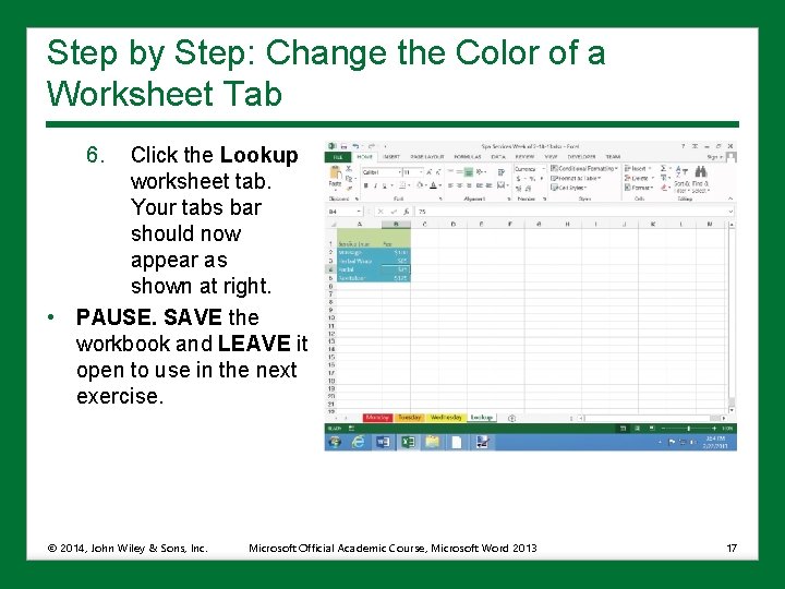
Step by Step: Change the Color of a Worksheet Tab 6. Click the Lookup worksheet tab. Your tabs bar should now appear as shown at right. • PAUSE. SAVE the workbook and LEAVE it open to use in the next exercise. © 2014, John Wiley & Sons, Inc. Microsoft Official Academic Course, Microsoft Word 2013 17

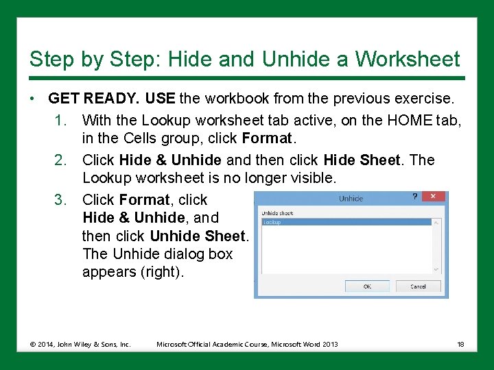
Step by Step: Hide and Unhide a Worksheet • GET READY. USE the workbook from the previous exercise. 1. With the Lookup worksheet tab active, on the HOME tab, in the Cells group, click Format. 2. Click Hide & Unhide and then click Hide Sheet. The Lookup worksheet is no longer visible. 3. Click Format, click Hide & Unhide, and then click Unhide Sheet. The Unhide dialog box appears (right). © 2014, John Wiley & Sons, Inc. Microsoft Official Academic Course, Microsoft Word 2013 18

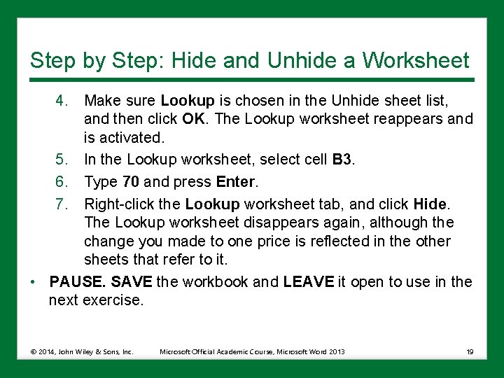
Step by Step: Hide and Unhide a Worksheet 4. Make sure Lookup is chosen in the Unhide sheet list, and then click OK. The Lookup worksheet reappears and is activated. 5. In the Lookup worksheet, select cell B 3. 6. Type 70 and press Enter. 7. Right-click the Lookup worksheet tab, and click Hide. The Lookup worksheet disappears again, although the change you made to one price is reflected in the other sheets that refer to it. • PAUSE. SAVE the workbook and LEAVE it open to use in the next exercise. © 2014, John Wiley & Sons, Inc. Microsoft Official Academic Course, Microsoft Word 2013 19

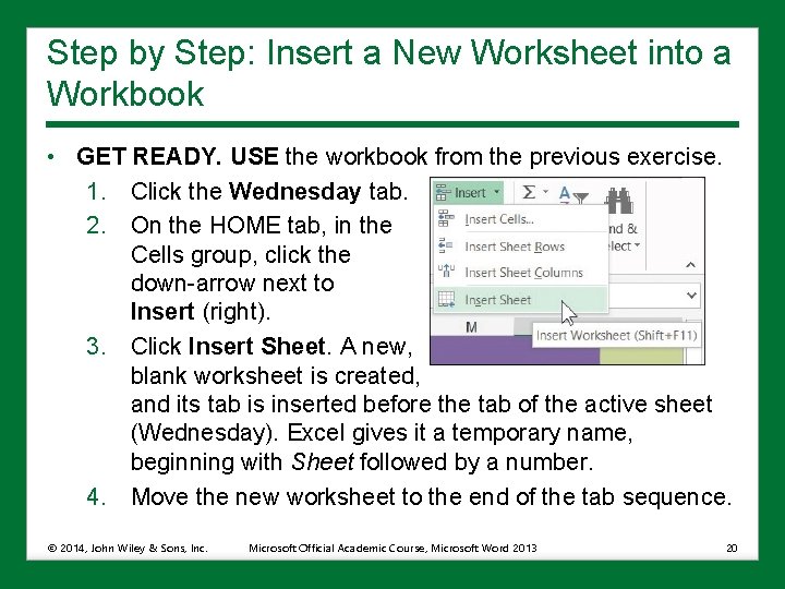
Step by Step: Insert a New Worksheet into a Workbook • GET READY. USE the workbook from the previous exercise. 1. Click the Wednesday tab. 2. On the HOME tab, in the Cells group, click the down-arrow next to Insert (right). 3. Click Insert Sheet. A new, blank worksheet is created, and its tab is inserted before the tab of the active sheet (Wednesday). Excel gives it a temporary name, beginning with Sheet followed by a number. 4. Move the new worksheet to the end of the tab sequence. © 2014, John Wiley & Sons, Inc. Microsoft Official Academic Course, Microsoft Word 2013 20

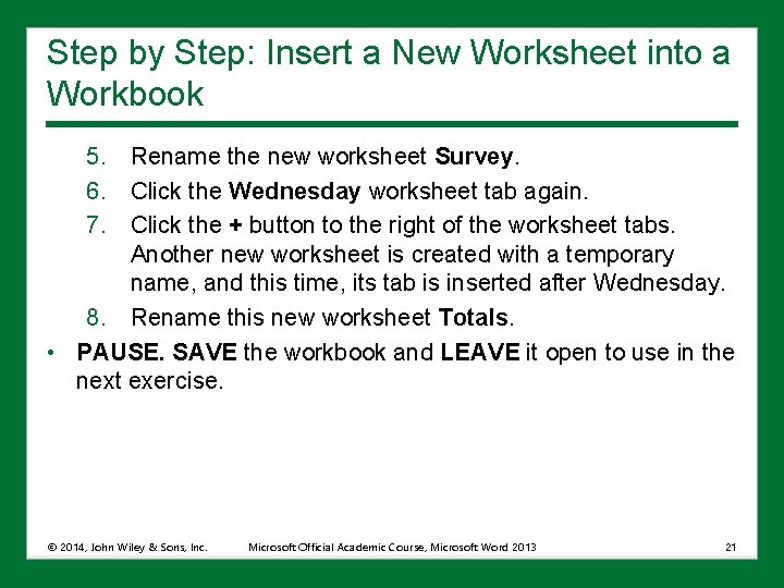
Step by Step: Insert a New Worksheet into a Workbook 5. Rename the new worksheet Survey. 6. Click the Wednesday worksheet tab again. 7. Click the + button to the right of the worksheet tabs. Another new worksheet is created with a temporary name, and this time, its tab is inserted after Wednesday. 8. Rename this new worksheet Totals. • PAUSE. SAVE the workbook and LEAVE it open to use in the next exercise. © 2014, John Wiley & Sons, Inc. Microsoft Official Academic Course, Microsoft Word 2013 21

Step by Step: Delete a Worksheet from a Workbook • GET READY. USE the workbook from the previous exercise. 1. Click the Totals worksheet tab. 2. On the HOME table, in the Cells group, click the downarrow next to Delete. 3. Click Delete Sheet. The Totals worksheet is removed and its tab disappears. 4. Right-click the Survey tab, and click Delete. The Survey worksheet is removed and its tab disappears. • PAUSE. SAVE the workbook and LEAVE it open to use in the next exercise. © 2014, John Wiley & Sons, Inc. Microsoft Official Academic Course, Microsoft Word 2013 22

Step by Step: Work with Multiple Worksheets in a Workbook • GET READY. USE the workbook from the previous exercise. 1. SAVE the workbook in the Lesson 8 folder as 08 Spa Services Week of 2 -18 -13 Solution 2. 2. Right-click any worksheet’s tab and click Select All Sheets. The title bar now reads Spa Services Week of 218 -13. xlsx [Group]. All visible worksheets are enrolled in this group, whereas hidden worksheets are excluded. Although all the worksheets’ tabs are now boldface, the active worksheet remains highlighted in green. 3. Select cells I 8: M 33. © 2014, John Wiley & Sons, Inc. Microsoft Official Academic Course, Microsoft Word 2013 23

Step by Step: Work with Multiple Worksheets in a Workbook 4. Click $ (Accounting Number Format) in the Number group of the Home menu tab. The cell formats for the range switch to a currency style where the dollar sign is aligned left, and the value aligned right with dollars and cents. Column K (Facial) is too narrow for its contents, so its values currently read ####. 5. v. Adjust the width of column K to fit its contents (see Lesson 7, “Formatting Worksheets”). 6. Select column M. 7. In the Font group, click B (Bold). All cells in column M are now boldfaced. © 2014, John Wiley & Sons, Inc. Microsoft Official Academic Course, Microsoft Word 2013 24

Step by Step: Work with Multiple Worksheets in a Workbook 8. Click the tab for a worksheet other than Wednesday. The group is now dissolved, but the changes you made to the previous sheet are reflected here, as demonstrated by the reformatted Wednesday worksheet shown below. 9. Select the Monday worksheet. © 2014, John Wiley & Sons, Inc. Microsoft Official Academic Course, Microsoft Word 2013 25

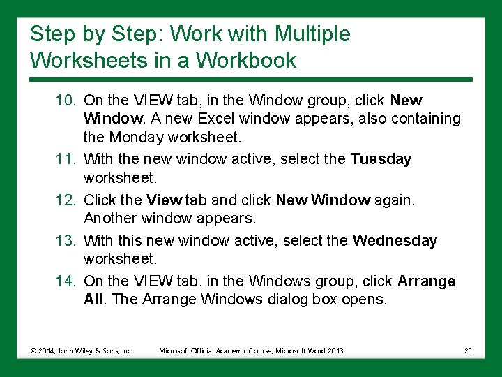
Step by Step: Work with Multiple Worksheets in a Workbook 10. On the VIEW tab, in the Window group, click New Window. A new Excel window appears, also containing the Monday worksheet. 11. With the new window active, select the Tuesday worksheet. 12. Click the View tab and click New Window again. Another window appears. 13. With this new window active, select the Wednesday worksheet. 14. On the VIEW tab, in the Windows group, click Arrange All. The Arrange Windows dialog box opens. © 2014, John Wiley & Sons, Inc. Microsoft Official Academic Course, Microsoft Word 2013 26

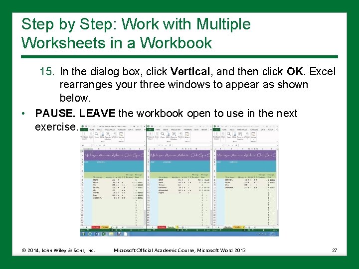
Step by Step: Work with Multiple Worksheets in a Workbook 15. In the dialog box, click Vertical, and then click OK. Excel rearranges your three windows to appear as shown below. • PAUSE. LEAVE the workbook open to use in the next exercise. © 2014, John Wiley & Sons, Inc. Microsoft Official Academic Course, Microsoft Word 2013 27

Step by Step: Hide and Unhide Worksheet Windows in a Workbook • GET READY. USE the workbook from the previous exercise. 1. With all three non-hidden worksheets visible, click the title bar of the window containing the Monday worksheet. 2. On the VIEW tab, in the Window group, click Hide. The Monday window is closed. 3. In either of the visible windows, on the VIEW tab, in the Window group, click Unhide. The Unhide dialog box appears. 4. In the Unhide workbook list, choose the hidden window and click OK. • PAUSE. SAVE the workbook and LEAVE it open to use in the next exercise. © 2014, John Wiley & Sons, Inc. Microsoft Official Academic Course, Microsoft Word 2013 28

Step by Step: Use Zoom and Freeze to Change the Onscreen View • GET READY. USE the workbook from the previous exercise. 1. SAVE the workbook in the Lesson 8 folder as 08 Spa Services Week of 2 -18 -13 Solution 3. 2. Maximize the window containing the Monday worksheet. 3. Select cell B 8. © 2014, John Wiley & Sons, Inc. Microsoft Official Academic Course, Microsoft Word 2013 29

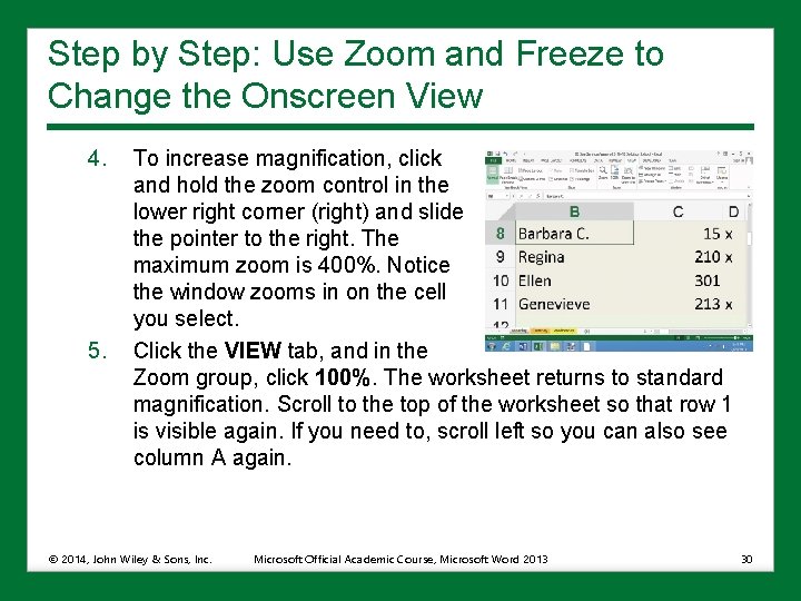
Step by Step: Use Zoom and Freeze to Change the Onscreen View 4. 5. To increase magnification, click and hold the zoom control in the lower right corner (right) and slide the pointer to the right. The maximum zoom is 400%. Notice the window zooms in on the cell you select. Click the VIEW tab, and in the Zoom group, click 100%. The worksheet returns to standard magnification. Scroll to the top of the worksheet so that row 1 is visible again. If you need to, scroll left so you can also see column A again. © 2014, John Wiley & Sons, Inc. Microsoft Official Academic Course, Microsoft Word 2013 30

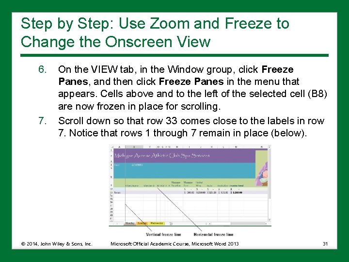
Step by Step: Use Zoom and Freeze to Change the Onscreen View 6. 7. On the VIEW tab, in the Window group, click Freeze Panes, and then click Freeze Panes in the menu that appears. Cells above and to the left of the selected cell (B 8) are now frozen in place for scrolling. Scroll down so that row 33 comes close to the labels in row 7. Notice that rows 1 through 7 remain in place (below). © 2014, John Wiley & Sons, Inc. Microsoft Official Academic Course, Microsoft Word 2013 31

Step by Step: Use Zoom and Freeze to Change the Onscreen View 8. Press Ctrl + Home to scroll the worksheet to the top. In the Window group, click Freeze Panes, and then click Unfreeze Panes. The thin lines denoting the frozen borders of the worksheet disappear. • PAUSE. LEAVE the workbook open to use in the next exercise. © 2014, John Wiley & Sons, Inc. Microsoft Official Academic Course, Microsoft Word 2013 32

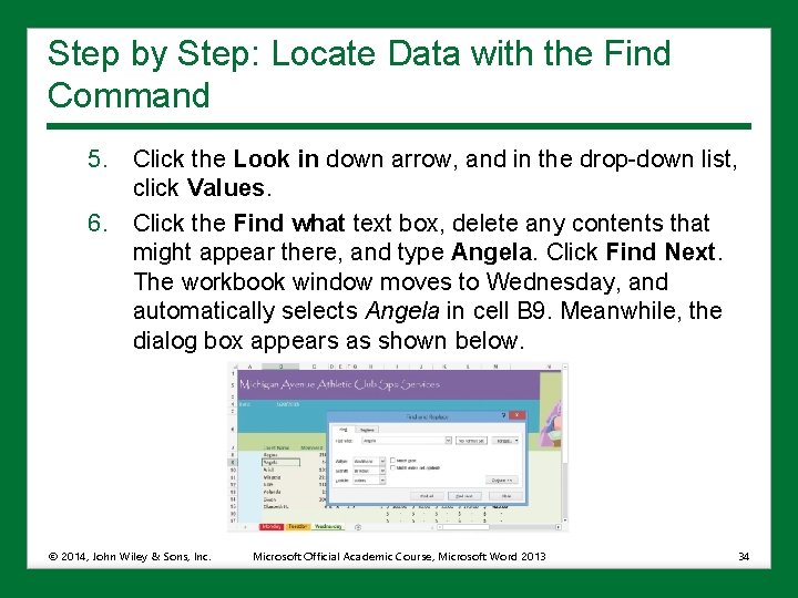
Step by Step: Locate Data with the Find Command • GET READY. USE the workbook from the previous exercise. 1. Select the Monday worksheet. Select cell B 8. 2. On the HOME tab, in the Editing group, click Find & Select (the binoculars button). Click Find. The Find and Replace dialog box appears. 3. In the dialog box, click Options. The dialog box expands. 4. Click the Within down arrow, and in the drop-down list, click Workbook. © 2014, John Wiley & Sons, Inc. Microsoft Official Academic Course, Microsoft Word 2013 33

Step by Step: Locate Data with the Find Command 5. Click the Look in down arrow, and in the drop-down list, click Values. 6. Click the Find what text box, delete any contents that might appear there, and type Angela. Click Find Next. The workbook window moves to Wednesday, and automatically selects Angela in cell B 9. Meanwhile, the dialog box appears as shown below. © 2014, John Wiley & Sons, Inc. Microsoft Official Academic Course, Microsoft Word 2013 34

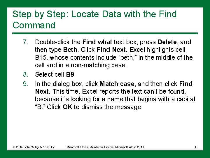
Step by Step: Locate Data with the Find Command 7. Double-click the Find what text box, press Delete, and then type Beth. Click Find Next. Excel highlights cell B 15, whose contents include “beth, ” in the middle of the cell and in a non-matching case. 8. Select cell B 9. 9. In the dialog box, click Match case, and then click Find Next. This time, Excel reports the text can’t be found, because it’s looking for a name that begins with a capital “B. ” Click OK to dismiss the message. © 2014, John Wiley & Sons, Inc. Microsoft Official Academic Course, Microsoft Word 2013 35

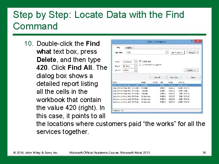
Step by Step: Locate Data with the Find Command 10. Double-click the Find what text box, press Delete, and then type 420. Click Find All. The dialog box shows a detailed report listing all the cells in the workbook that contain the value 420 (right). In this case, it points to all the locations where customers paid “the works” for all the services together. © 2014, John Wiley & Sons, Inc. Microsoft Official Academic Course, Microsoft Word 2013 36

Step by Step: Locate Data with the Find Command 11. Click the first item in the list whose Sheet entry is marked Tuesday. Excel brings up the Tuesday worksheet and selects cell M 9, which contains an entry for $420. 00. 12. Click Close to dismiss the dialog box. 13. Close the other two open workbook windows. • PAUSE. LEAVE the workbook open to use in the next exercise. © 2014, John Wiley & Sons, Inc. Microsoft Official Academic Course, Microsoft Word 2013 37

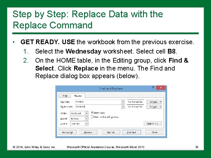
Step by Step: Replace Data with the Replace Command • GET READY. USE the workbook from the previous exercise. 1. Select the Wednesday worksheet. Select cell B 8. 2. On the HOME table, in the Editing group, click Find & Select. Click Replace in the menu. The Find and Replace dialog box appears (below). © 2014, John Wiley & Sons, Inc. Microsoft Official Academic Course, Microsoft Word 2013 38

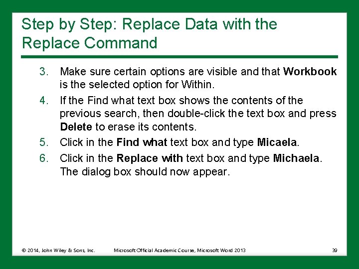
Step by Step: Replace Data with the Replace Command 3. Make sure certain options are visible and that Workbook is the selected option for Within. 4. If the Find what text box shows the contents of the previous search, then double-click the text box and press Delete to erase its contents. 5. Click in the Find what text box and type Micaela. 6. Click in the Replace with text box and type Michaela. The dialog box should now appear. © 2014, John Wiley & Sons, Inc. Microsoft Official Academic Course, Microsoft Word 2013 39

Step by Step: Replace Data with the Replace Command 7. Click Replace All. Excel searches for all instances of Micaela and adds an “h” to the middle (correcting this client’s spelling), and then will notify you when the job is done. Excel makes one replacement. 8. Click OK, and then click Close. • SAVE the workbook, and LEAVE it open to use in the next exercise. © 2014, John Wiley & Sons, Inc. Microsoft Official Academic Course, Microsoft Word 2013 40

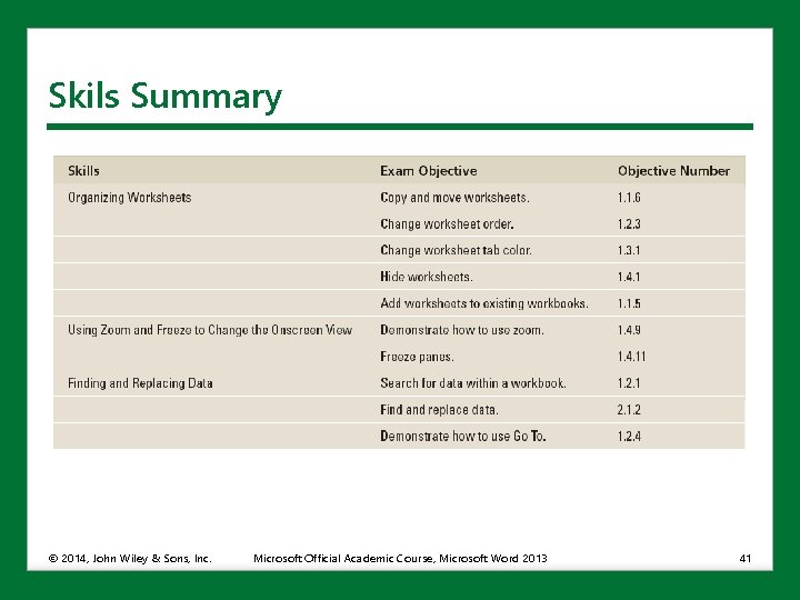
Skils Summary © 2014, John Wiley & Sons, Inc. Microsoft Official Academic Course, Microsoft Word 2013 41