Microsoft Excel 2013 Lesson 7 Formatting Worksheets 2014

Microsoft Excel 2013 Lesson 7 Formatting Worksheets © 2014, John Wiley & Sons, Inc. Microsoft Official Academic Course, Microsoft Word 2013 1

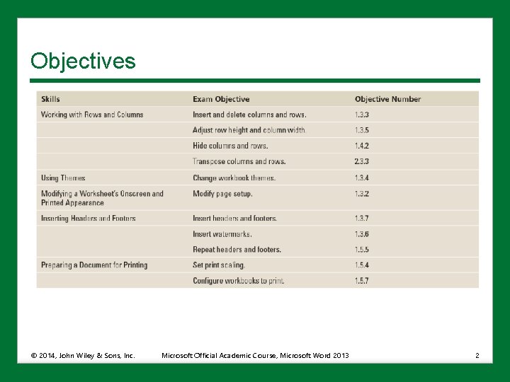
Objectives © 2014, John Wiley & Sons, Inc. Microsoft Official Academic Course, Microsoft Word 2013 2

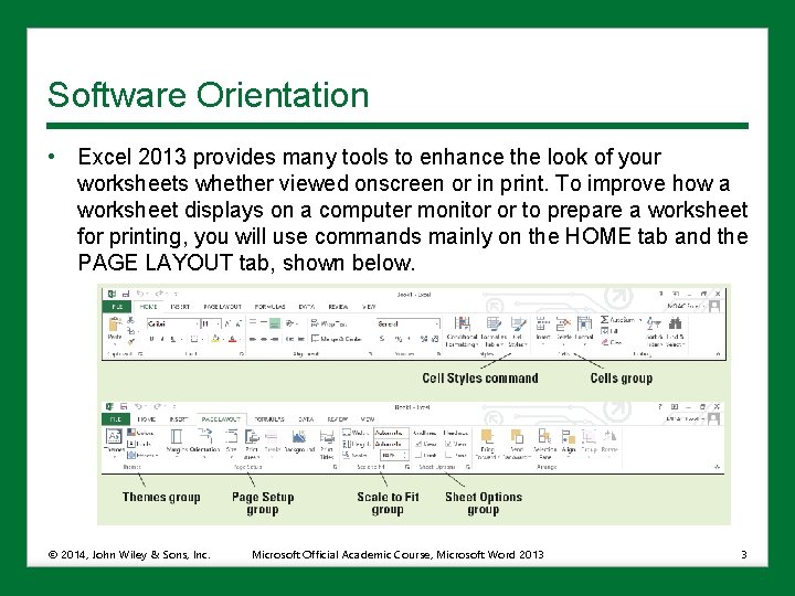
Software Orientation • Excel 2013 provides many tools to enhance the look of your worksheets whether viewed onscreen or in print. To improve how a worksheet displays on a computer monitor or to prepare a worksheet for printing, you will use commands mainly on the HOME tab and the PAGE LAYOUT tab, shown below. © 2014, John Wiley & Sons, Inc. Microsoft Official Academic Course, Microsoft Word 2013 3

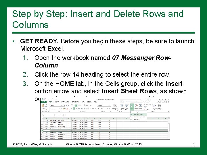
Step by Step: Insert and Delete Rows and Columns • GET READY. Before you begin these steps, be sure to launch Microsoft Excel. 1. Open the workbook named 07 Messenger Row. Column. 2. Click the row 14 heading to select the entire row. 3. On the HOME tab, in the Cells group, click the Insert button arrow and select Insert Sheet Rows, as shown below. A new blank row appears as row 14. © 2014, John Wiley & Sons, Inc. Microsoft Official Academic Course, Microsoft Word 2013 4

Step by Step: Insert and Delete Rows and Columns 4. To insert several rows at once, click the row 25 heading, hold down the Ctrl key, and then click row headings 34 and 43. Right-click any of the selected rows and select Insert from the shortcut menu. Blank rows appear above the selected rows, so that data for each messenger is separated by a blank row. 5. Click the column D heading to select the entire column. This column contains the delivery zone. 6. On the HOME tab, in the Cells group, click the Delete button arrow and select Delete Sheet Columns. The Zone column disappears. © 2014, John Wiley & Sons, Inc. Microsoft Official Academic Course, Microsoft Word 2013 5

Step by Step: Insert and Delete Rows and Columns 7. Right-click the row 3 heading and select Insert from the shortcut menu. In cell A 3, type Zone 1. 8. Select A 3: I 3. On the HOME tab, in the Alignment group, click the Merge & Center button. The “Zone 1” text is centered across the data columns. 9. SAVE the workbook. • PAUSE. Leave the workbook open to use in the next exercise. © 2014, John Wiley & Sons, Inc. Microsoft Official Academic Course, Microsoft Word 2013 6

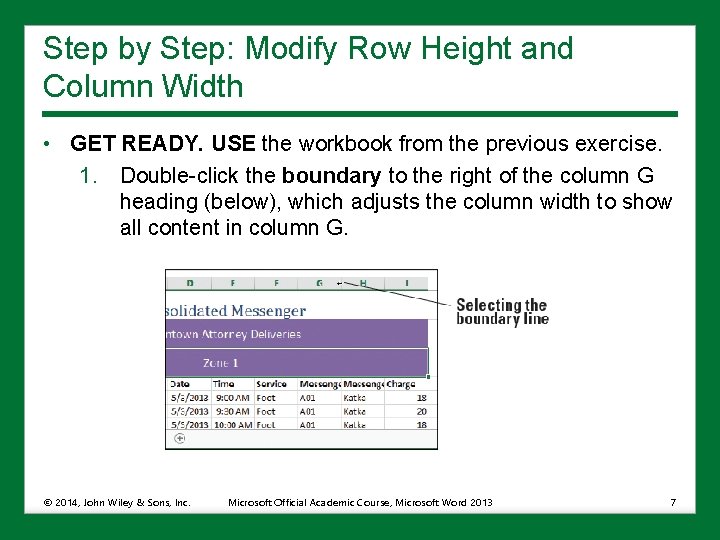
Step by Step: Modify Row Height and Column Width • GET READY. USE the workbook from the previous exercise. 1. Double-click the boundary to the right of the column G heading (below), which adjusts the column width to show all content in column G. © 2014, John Wiley & Sons, Inc. Microsoft Official Academic Course, Microsoft Word 2013 7

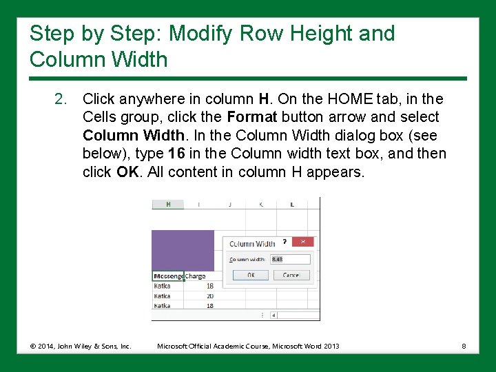
Step by Step: Modify Row Height and Column Width 2. Click anywhere in column H. On the HOME tab, in the Cells group, click the Format button arrow and select Column Width. In the Column Width dialog box (see below), type 16 in the Column width text box, and then click OK. All content in column H appears. © 2014, John Wiley & Sons, Inc. Microsoft Official Academic Course, Microsoft Word 2013 8

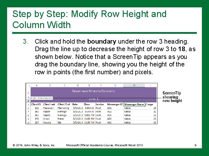
Step by Step: Modify Row Height and Column Width 3. Click and hold the boundary under the row 3 heading. Drag the line up to decrease the height of row 3 to 18, as shown below. Notice that a Screen. Tip appears as you drag the boundary line, showing you the height of the row in points (the first number) and pixels. © 2014, John Wiley & Sons, Inc. Microsoft Official Academic Course, Microsoft Word 2013 9

Step by Step: Modify Row Height and Column Width 4. Select row 2. On the HOME tab, in the Cells group, click the Format button arrow and select Auto. Fit Row Height. With the row still selected, click the Format button arrow again and select Row Height. The Row Height dialog box indicates that the row is 18. 75 points in height. Click OK. 5. SAVE the workbook. • PAUSE. Leave the workbook open to use in the next exercise. © 2014, John Wiley & Sons, Inc. Microsoft Official Academic Course, Microsoft Word 2013 10

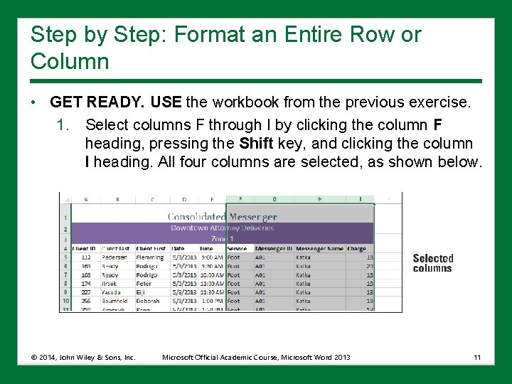
Step by Step: Format an Entire Row or Column • GET READY. USE the workbook from the previous exercise. 1. Select columns F through I by clicking the column F heading, pressing the Shift key, and clicking the column I heading. All four columns are selected, as shown below. © 2014, John Wiley & Sons, Inc. Microsoft Official Academic Course, Microsoft Word 2013 11

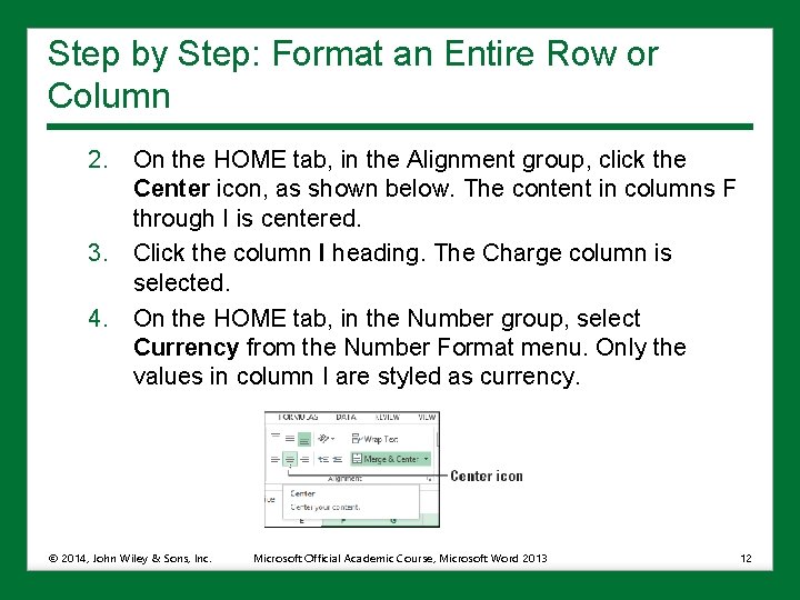
Step by Step: Format an Entire Row or Column 2. On the HOME tab, in the Alignment group, click the Center icon, as shown below. The content in columns F through I is centered. 3. Click the column I heading. The Charge column is selected. 4. On the HOME tab, in the Number group, select Currency from the Number Format menu. Only the values in column I are styled as currency. © 2014, John Wiley & Sons, Inc. Microsoft Official Academic Course, Microsoft Word 2013 12

Step by Step: Format an Entire Row or Column 5. Select row 4 and center the column headings using the Center icon in the Alignment group on the HOME tab. 6. SAVE the workbook. • PAUSE. Leave the workbook open to use in the next exercise. . © 2014, John Wiley & Sons, Inc. Microsoft Official Academic Course, Microsoft Word 2013 13

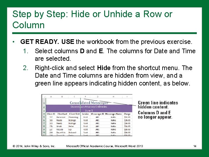
Step by Step: Hide or Unhide a Row or Column • GET READY. USE the workbook from the previous exercise. 1. Select columns D and E. The columns for Date and Time are selected. 2. Right-click and select Hide from the shortcut menu. The Date and Time columns are hidden from view, and a green line appears indicating hidden content, as below. © 2014, John Wiley & Sons, Inc. Microsoft Official Academic Course, Microsoft Word 2013 14

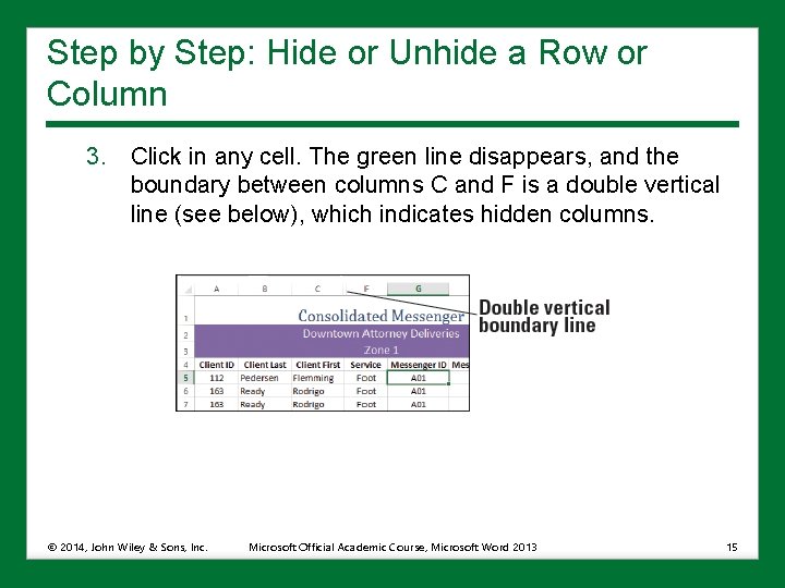
Step by Step: Hide or Unhide a Row or Column 3. Click in any cell. The green line disappears, and the boundary between columns C and F is a double vertical line (see below), which indicates hidden columns. © 2014, John Wiley & Sons, Inc. Microsoft Official Academic Course, Microsoft Word 2013 15

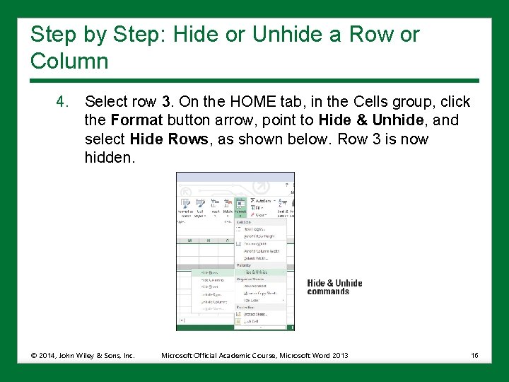
Step by Step: Hide or Unhide a Row or Column 4. Select row 3. On the HOME tab, in the Cells group, click the Format button arrow, point to Hide & Unhide, and select Hide Rows, as shown below. Row 3 is now hidden. © 2014, John Wiley & Sons, Inc. Microsoft Official Academic Course, Microsoft Word 2013 16

Step by Step: Hide or Unhide a Row or Column 5. Select rows 2 and 4. Right-click the selection and select Unhide from the shortcut menu. Row 3 is now visible. • PAUSE. Leave the workbook open to use in the next exercise. © 2014, John Wiley & Sons, Inc. Microsoft Official Academic Course, Microsoft Word 2013 17

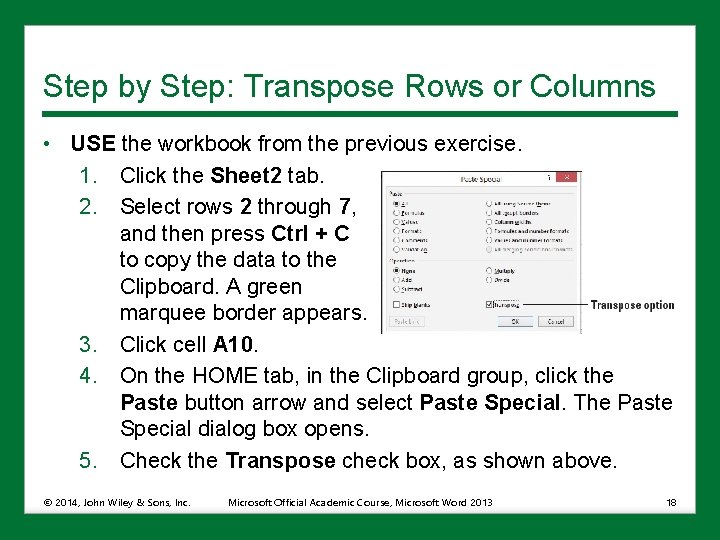
Step by Step: Transpose Rows or Columns • USE the workbook from the previous exercise. 1. Click the Sheet 2 tab. 2. Select rows 2 through 7, and then press Ctrl + C to copy the data to the Clipboard. A green marquee border appears. 3. Click cell A 10. 4. On the HOME tab, in the Clipboard group, click the Paste button arrow and select Paste Special. The Paste Special dialog box opens. 5. Check the Transpose check box, as shown above. © 2014, John Wiley & Sons, Inc. Microsoft Official Academic Course, Microsoft Word 2013 18

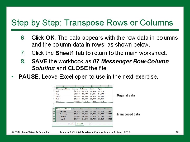
Step by Step: Transpose Rows or Columns 6. Click OK. The data appears with the row data in columns and the column data in rows, as shown below. 7. Click the Sheet 1 tab to return to the main worksheet. 8. SAVE the workbook as 07 Messenger Row-Column Solution and CLOSE the file. • PAUSE. Leave Excel open to use in the next exercise. © 2014, John Wiley & Sons, Inc. Microsoft Official Academic Course, Microsoft Word 2013 19

Step by Step: Choose a Theme for a Workbook • GET READY. LAUNCH Excel if it is not already running. 1. OPEN the 07 Messenger Theme data file for this lesson. 2. With Sheet 1 active, click cell A 3. 3. On the HOME tab, in the Styles group, click the Cell Styles button arrow and select 20% - Accent 4. A light purple background is applied to the cell range, the font size is reduced, and the font color changes to black. 4. On the PAGE LAYOUT tab, in the Themes group, click the Themes button arrow to open the Themes gallery. Several built-in themes appear in the gallery. Move your mouse pointer over each theme to see its effect on the underlying worksheet, which is referred to as Live © 2014, John Wiley & Sons, Inc. 20 Preview. Microsoft Official Academic Course, Microsoft Word 2013

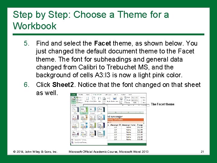
Step by Step: Choose a Theme for a Workbook 5. Find and select the Facet theme, as shown below. You just changed the default document theme to the Facet theme. The font for subheadings and general data changed from Calibri to Trebuchet MS, and the background of cells A 3: I 3 is now a light pink color. 6. Click Sheet 2. Notice that the font changed on that sheet as well. © 2014, John Wiley & Sons, Inc. Microsoft Official Academic Course, Microsoft Word 2013 21

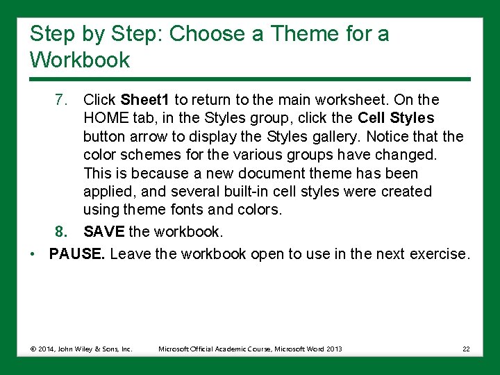
Step by Step: Choose a Theme for a Workbook 7. Click Sheet 1 to return to the main worksheet. On the HOME tab, in the Styles group, click the Cell Styles button arrow to display the Styles gallery. Notice that the color schemes for the various groups have changed. This is because a new document theme has been applied, and several built-in cell styles were created using theme fonts and colors. 8. SAVE the workbook. • PAUSE. Leave the workbook open to use in the next exercise. © 2014, John Wiley & Sons, Inc. Microsoft Official Academic Course, Microsoft Word 2013 22

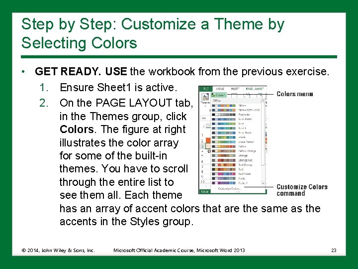
Step by Step: Customize a Theme by Selecting Colors • GET READY. USE the workbook from the previous exercise. 1. Ensure Sheet 1 is active. 2. On the PAGE LAYOUT tab, in the Themes group, click Colors. The figure at right illustrates the color array for some of the built-in themes. You have to scroll through the entire list to see them all. Each theme has an array of accent colors that are the same as the accents in the Styles group. © 2014, John Wiley & Sons, Inc. Microsoft Official Academic Course, Microsoft Word 2013 23

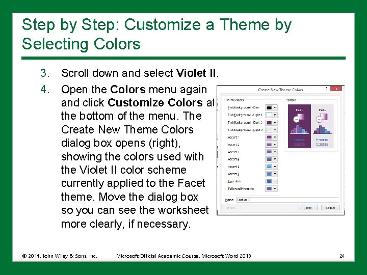
Step by Step: Customize a Theme by Selecting Colors 3. Scroll down and select Violet II. 4. Open the Colors menu again and click Customize Colors at the bottom of the menu. The Create New Theme Colors dialog box opens (right), showing the colors used with the Violet II color scheme currently applied to the Facet theme. Move the dialog box so you can see the worksheet more clearly, if necessary. © 2014, John Wiley & Sons, Inc. Microsoft Official Academic Course, Microsoft Word 2013 24

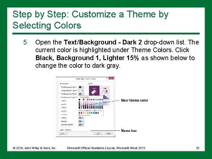
Step by Step: Customize a Theme by Selecting Colors 5. Open the Text/Background - Dark 2 drop-down list. The current color is highlighted under Theme Colors. Click Black, Background 1, Lighter 15% as shown below to change the color to dark gray. © 2014, John Wiley & Sons, Inc. Microsoft Official Academic Course, Microsoft Word 2013 25

Step by Step: Customize a Theme by Selecting Colors 6. In the Name box at the bottom of the dialog box, type Consolidated Messenger and click Save. The new text color is reflected in row 1. If you want to modify colors for Consolidated Messenger in the future, just modify the Consolidated Messenger color scheme, which appears at the top of the Colors menu. 7. SAVE the workbook. • PAUSE. Leave the workbook open to use in the next exercise. © 2014, John Wiley & Sons, Inc. Microsoft Official Academic Course, Microsoft Word 2013 26

Step by Step: Customize a Theme by Selecting Fonts and Effects • GET READY. USE the workbook from the previous exercise. 1. With Sheet 1 active, on the PAGE LAYOUT tab, in the Themes group, click Fonts. 2. Click Customize Fonts. The Create New Theme Fonts dialog box opens. 3. Open the Heading font drop-down menu, locate the Arial font, and select it. 4. In the Body font box, locate and select Arial Narrow. The preview in the Sample box is updated with the fonts that you selected. © 2014, John Wiley & Sons, Inc. Microsoft Official Academic Course, Microsoft Word 2013 27

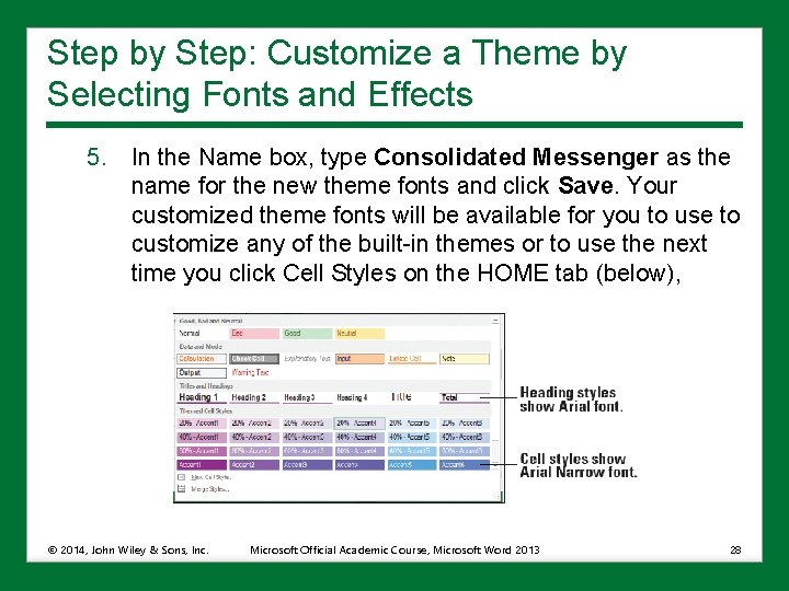
Step by Step: Customize a Theme by Selecting Fonts and Effects 5. In the Name box, type Consolidated Messenger as the name for the new theme fonts and click Save. Your customized theme fonts will be available for you to use to customize any of the built-in themes or to use the next time you click Cell Styles on the HOME tab (below), © 2014, John Wiley & Sons, Inc. Microsoft Official Academic Course, Microsoft Word 2013 28

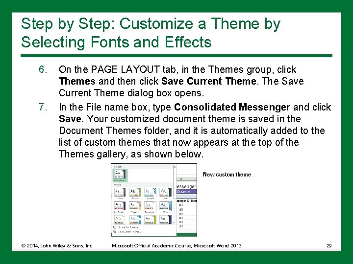
Step by Step: Customize a Theme by Selecting Fonts and Effects 6. 7. On the PAGE LAYOUT tab, in the Themes group, click Themes and then click Save Current Theme. The Save Current Theme dialog box opens. In the File name box, type Consolidated Messenger and click Save. Your customized document theme is saved in the Document Themes folder, and it is automatically added to the list of custom themes that now appears at the top of the Themes gallery, as shown below. © 2014, John Wiley & Sons, Inc. Microsoft Official Academic Course, Microsoft Word 2013 29

Step by Step: Customize a Theme by Selecting Fonts and Effects 8. On the PAGE LAYOUT tab, in the Themes group, click Effects. Theme effects are sets of lines and fill effects. Hovering your mouse over the effects will show subtle changes in the cells; however, you will notice the result of changing an effect only if you have charts, shapes, Smart. Art, or similar graphics in your workbook. 9. Click the Reflection effect to apply it to the workbook. Click Undo in the Quick Access Toolbar to undo theme effect. 10. SAVE the workbook as 07 Messenger Theme Solution and CLOSE the file. • PAUSE. Leave Excel open to use in the next exercise. © 2014, John Wiley & Sons, Inc. Microsoft Official Academic Course, Microsoft Word 2013 30

Step by Step: Format a Worksheet Background • GET READY. LAUNCH Excel if it is not already running. 1. OPEN the 07 Messenger Appearance data file for this lesson. 2. Ensure Sheet 1 is active. 3. On the PAGE LAYOUT tab, in the Page Setup group, click the Background button. The Insert Pictures dialog box opens. 4. Click Browse next to From a file. The Sheet Background dialog box opens. 5. Navigate to the student data files folder, select 07 bike_courier. jpg, and then click Insert. The selected picture is displayed behind the © 2014, John Wiley & Sons, Inc. Microsoft Official Academic Course, Microsoft Word 2013 31

Step by Step: Format a Worksheet Background 6. On the PAGE LAYOUT tab, in the Page Setup group, click Delete Background. The background is removed. 7. SAVE the workbook. • PAUSE. Leave the workbook open to use in the next exercise. © 2014, John Wiley & Sons, Inc. Microsoft Official Academic Course, Microsoft Word 2013 32

Step by Step: View and Print a Worksheet’s Gridlines • GET READY. USE the workbook from the previous exercise. 1. Ensure Sheet 1 is active. 2. On the PAGE LAYOUT tab, in the Sheet Options group, uncheck the Gridlines View check box. The gridlines disappear from the worksheet. 3. Check the Gridlines View check box to restore viewable gridlines. © 2014, John Wiley & Sons, Inc. Microsoft Official Academic Course, Microsoft Word 2013 33

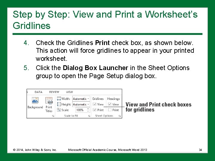
Step by Step: View and Print a Worksheet’s Gridlines 4. Check the Gridlines Print check box, as shown below. This action will force gridlines to appear in your printed worksheet. 5. Click the Dialog Box Launcher in the Sheet Options group to open the Page Setup dialog box. © 2014, John Wiley & Sons, Inc. Microsoft Official Academic Course, Microsoft Word 2013 34

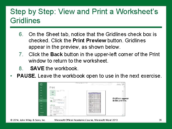
Step by Step: View and Print a Worksheet’s Gridlines 6. On the Sheet tab, notice that the Gridlines check box is checked. Click the Print Preview button. Gridlines appear in the preview, as shown below. 7. Click the Back button in the upper-left corner of the Print window to return to the worksheet. 8. SAVE the workbook. • PAUSE. Leave the workbook open to use in the next exercise. © 2014, John Wiley & Sons, Inc. Microsoft Official Academic Course, Microsoft Word 2013 35

Step by Step: View and Print Column and Row Headings • GET READY. USE the workbook from the previous exercise. 1. Ensure Sheet 1 is active. 2. On the PAGE LAYOUT tab, in the Sheet Options group, uncheck the Headings View check box. The row and column headings disappear from the worksheet. 3. Check the Headings View check box to restore the row and column headings. 4. Check the Headings Print check box. This action will force row and column headings to appear in your printed worksheet. 5. Click the Dialog Box Launcher in the Sheet Options group to open the Page Setup dialog box. © 2014, John Wiley & Sons, Inc. Microsoft Official Academic Course, Microsoft Word 2013 36

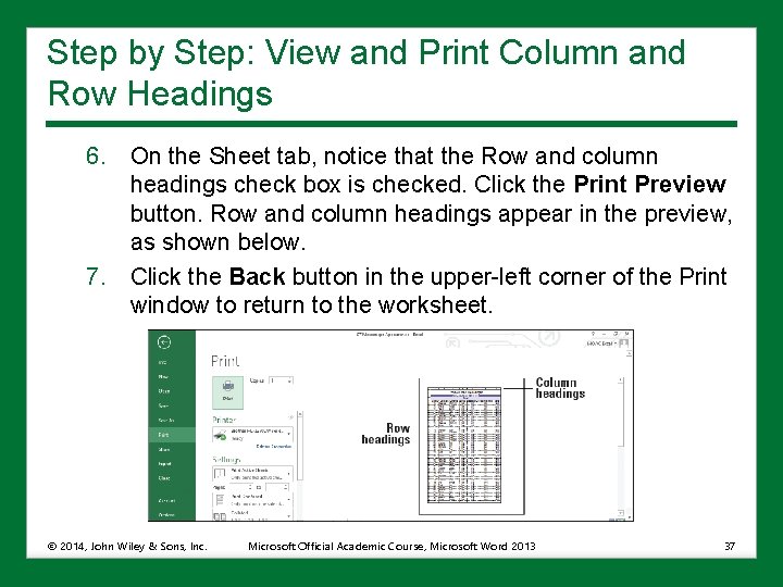
Step by Step: View and Print Column and Row Headings 6. On the Sheet tab, notice that the Row and column headings check box is checked. Click the Print Preview button. Row and column headings appear in the preview, as shown below. 7. Click the Back button in the upper-left corner of the Print window to return to the worksheet. © 2014, John Wiley & Sons, Inc. Microsoft Official Academic Course, Microsoft Word 2013 37

Step by Step: View and Print Column and Row Headings 8. Uncheck the Headings Print check box in the Sheet Options group on the PAGE LAYOUT tab. 9. SAVE the workbook as 07 Messenger Appearance Solution. • PAUSE. Leave the workbook open to use in the next exercise © 2014, John Wiley & Sons, Inc. Microsoft Official Academic Course, Microsoft Word 2013 38

Step by Step: Add Page Numbers to a Worksheet • GET READY. LAUNCH Excel if it is not already running. 1. OPEN the 07 Messenger Header-Footer data file for this lesson. 2. Ensure Sheet 1 is active. © 2014, John Wiley & Sons, Inc. Microsoft Official Academic Course, Microsoft Word 2013 39

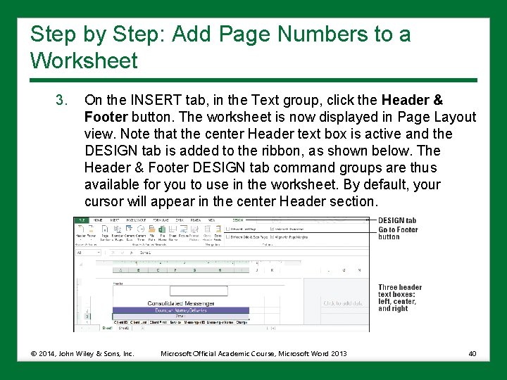
Step by Step: Add Page Numbers to a Worksheet 3. On the INSERT tab, in the Text group, click the Header & Footer button. The worksheet is now displayed in Page Layout view. Note that the center Header text box is active and the DESIGN tab is added to the ribbon, as shown below. The Header & Footer DESIGN tab command groups are thus available for you to use in the worksheet. By default, your cursor will appear in the center Header section. © 2014, John Wiley & Sons, Inc. Microsoft Official Academic Course, Microsoft Word 2013 40

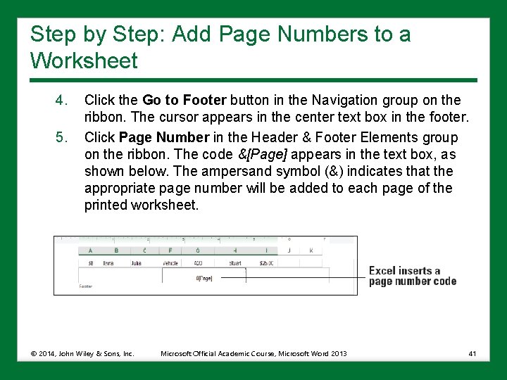
Step by Step: Add Page Numbers to a Worksheet 4. 5. Click the Go to Footer button in the Navigation group on the ribbon. The cursor appears in the center text box in the footer. Click Page Number in the Header & Footer Elements group on the ribbon. The code &[Page] appears in the text box, as shown below. The ampersand symbol (&) indicates that the appropriate page number will be added to each page of the printed worksheet. © 2014, John Wiley & Sons, Inc. Microsoft Official Academic Course, Microsoft Word 2013 41

Step by Step: Add Page Numbers to a Worksheet 6. Click in a worksheet cell that’s not part of the footer, and then click the Normal view icon on the right side of the status bar. 7. SAVE the workbook. • PAUSE. Leave the workbook open to use in the next exercise. © 2014, John Wiley & Sons, Inc. Microsoft Official Academic Course, Microsoft Word 2013 42

Step by Step: Insert a Predefined Header or Footer • GET READY. USE the workbook from the previous exercise. 1. Ensure Sheet 1 is active. Click cell A 1. 2. On the VIEW tab, in the Workbook Views group, click the Page Layout view button to view headers and footers. 3. Click the center header text box (which displays the “Click to add header” placeholder text). Click the Header & Footer Tools DESIGN tab now that it has become active. In the Header & Footer Elements group, click Sheet Name. &[Tab] appears in the text box. 4. In the Navigation group, click Go to Footer. Click the right footer text box. © 2014, John Wiley & Sons, Inc. Microsoft Official Academic Course, Microsoft Word 2013 43

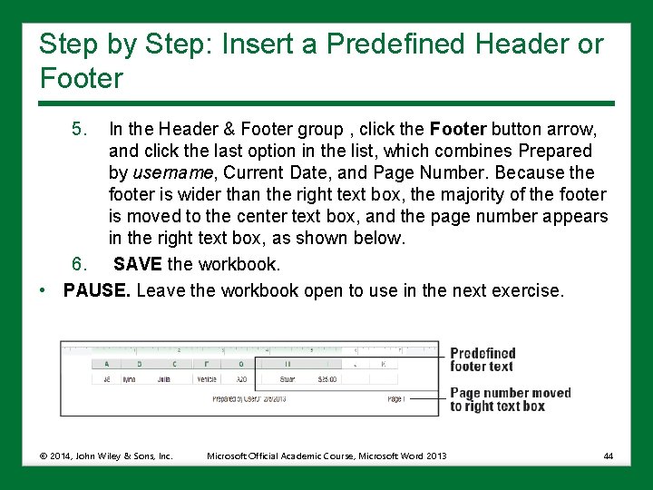
Step by Step: Insert a Predefined Header or Footer 5. In the Header & Footer group , click the Footer button arrow, and click the last option in the list, which combines Prepared by username, Current Date, and Page Number. Because the footer is wider than the right text box, the majority of the footer is moved to the center text box, and the page number appears in the right text box, as shown below. 6. SAVE the workbook. • PAUSE. Leave the workbook open to use in the next exercise. © 2014, John Wiley & Sons, Inc. Microsoft Official Academic Course, Microsoft Word 2013 44

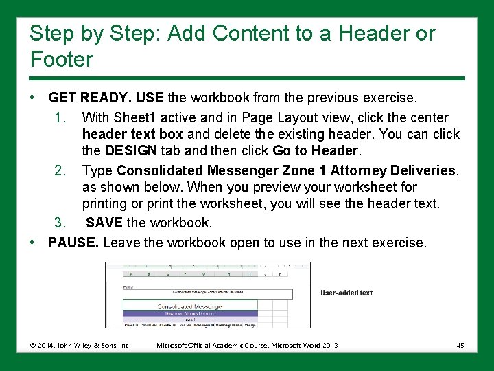
Step by Step: Add Content to a Header or Footer • GET READY. USE the workbook from the previous exercise. 1. With Sheet 1 active and in Page Layout view, click the center header text box and delete the existing header. You can click the DESIGN tab and then click Go to Header. 2. Type Consolidated Messenger Zone 1 Attorney Deliveries, as shown below. When you preview your worksheet for printing or print the worksheet, you will see the header text. 3. SAVE the workbook. • PAUSE. Leave the workbook open to use in the next exercise. © 2014, John Wiley & Sons, Inc. Microsoft Official Academic Course, Microsoft Word 2013 45

Step by Step: Insert a Watermark • GET READY. USE the workbook from the previous exercise. 1. Ensure Sheet 1 is active and in Page Layout view. 2. Click the left header text box. 3. On the DESIGN tab in the Header & Footer Elements group, click Picture. Click the Browse button, navigate to the student data files folder, select 07 watermark. gif, and then click Insert. Excel inserts an &[Picture] code into the left header text box. 4. Click outside of the header area, and then click the Normal view icon on the status bar. © 2014, John Wiley & Sons, Inc. Microsoft Official Academic Course, Microsoft Word 2013 46

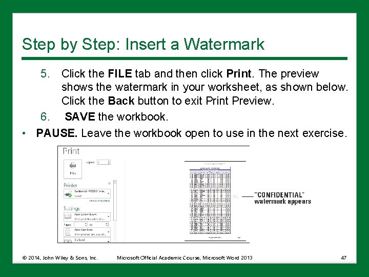
Step by Step: Insert a Watermark 5. Click the FILE tab and then click Print. The preview shows the watermark in your worksheet, as shown below. Click the Back button to exit Print Preview. 6. SAVE the workbook. • PAUSE. Leave the workbook open to use in the next exercise. © 2014, John Wiley & Sons, Inc. Microsoft Official Academic Course, Microsoft Word 2013 47

Step by Step: Repeat Headers and Footers • GET READY. USE the workbook from the previous exercise. 1. Ensure Sheet 1 is active and in Normal view. 2. On the PAGE LAYOUT tab, in the Page Setup group, click the Print Titles button. The Page Setup dialog box opens to the Sheet tab. 3. Type A 1: I 54 in the Print area text box. This is the range of all data on Sheet 1 to be printed. © 2014, John Wiley & Sons, Inc. Microsoft Official Academic Course, Microsoft Word 2013 48

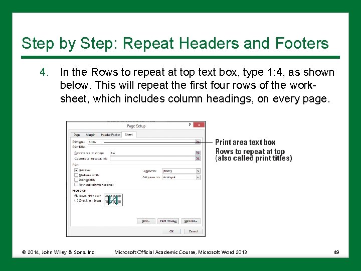
Step by Step: Repeat Headers and Footers 4. In the Rows to repeat at top text box, type 1: 4, as shown below. This will repeat the first four rows of the worksheet, which includes column headings, on every page. © 2014, John Wiley & Sons, Inc. Microsoft Official Academic Course, Microsoft Word 2013 49

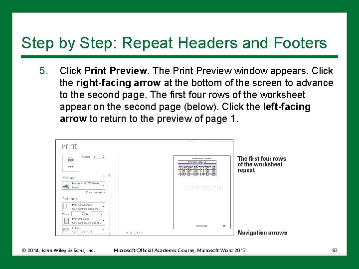
Step by Step: Repeat Headers and Footers 5. Click Print Preview. The Print Preview window appears. Click the right-facing arrow at the bottom of the screen to advance to the second page. The first four rows of the worksheet appear on the second page (below). Click the left-facing arrow to return to the preview of page 1. © 2014, John Wiley & Sons, Inc. Microsoft Official Academic Course, Microsoft Word 2013 50

Step by Step: Repeat Headers and Footers 6. 7. Click the Back button to return to the worksheet. SAVE the workbook as 07 Messenger Header-Footer Solution and CLOSE the file. • PAUSE. Leave Excel open to use in the next exercise. © 2014, John Wiley & Sons, Inc. Microsoft Official Academic Course, Microsoft Word 2013 51

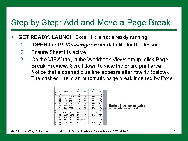
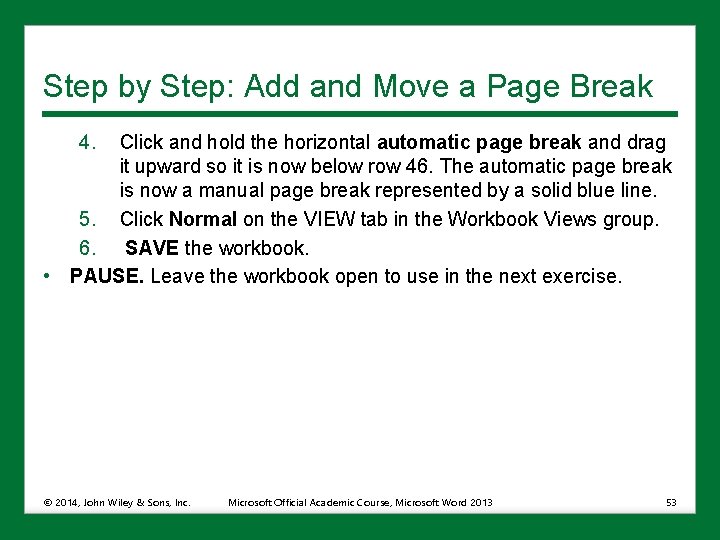
Step by Step: Add and Move a Page Break • GET READY. LAUNCH Excel if it is not already running. 1. OPEN the 07 Messenger Print data file for this lesson. 2. Ensure Sheet 1 is active. 3. On the VIEW tab, in the Workbook Views group, click Page Break Preview. Scroll down to view the entire print area. Notice that a dashed blue line appears after row 47 (below). The dashed line is an automatic page break inserted by Excel. © 2014, John Wiley & Sons, Inc. Microsoft Official Academic Course, Microsoft Word 2013 52

Step by Step: Add and Move a Page Break 4. Click and hold the horizontal automatic page break and drag it upward so it is now below row 46. The automatic page break is now a manual page break represented by a solid blue line. 5. Click Normal on the VIEW tab in the Workbook Views group. 6. SAVE the workbook. • PAUSE. Leave the workbook open to use in the next exercise. © 2014, John Wiley & Sons, Inc. Microsoft Official Academic Course, Microsoft Word 2013 53

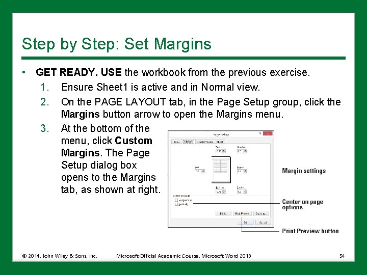
Step by Step: Set Margins • GET READY. USE the workbook from the previous exercise. 1. Ensure Sheet 1 is active and in Normal view. 2. On the PAGE LAYOUT tab, in the Page Setup group, click the Margins button arrow to open the Margins menu. 3. At the bottom of the menu, click Custom Margins. The Page Setup dialog box opens to the Margins tab, as shown at right. © 2014, John Wiley & Sons, Inc. Microsoft Official Academic Course, Microsoft Word 2013 54

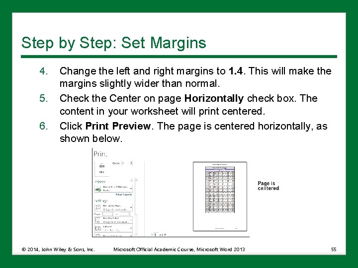
Step by Step: Set Margins 4. 5. 6. Change the left and right margins to 1. 4. This will make the margins slightly wider than normal. Check the Center on page Horizontally check box. The content in your worksheet will print centered. Click Print Preview. The page is centered horizontally, as shown below. © 2014, John Wiley & Sons, Inc. Microsoft Official Academic Course, Microsoft Word 2013 55

Step by Step: Set Margins 7. Click the Back button to leave Backstage. 8. SAVE the workbook. • PAUSE. Leave the workbook open to use in the next exercise. © 2014, John Wiley & Sons, Inc. Microsoft Official Academic Course, Microsoft Word 2013 56

Step by Step: Set a Worksheet’s Orientation • GET READY. USE the workbook from the previous exercise. 1. Ensure Sheet 1 is active and in Normal view. 2. On the PAGE LAYOUT tab, in the Page Setup group, click Orientation and then click Landscape. 3. Click the FILE tab, and then click Print. Click through the pages to see the worksheet in Landscape orientation. If you decided to keep this orientation, you would need to adjust page breaks to display all content properly. 4. Click the Back button to leave Backstage. 5. Repeat Step 2 to change the orientation back to Portrait. • PAUSE. Leave Excel open to use in the next exercise. © 2014, John Wiley & Sons, Inc. Microsoft Official Academic Course, Microsoft Word 2013 57

Step by Step: Scale a Worksheet to Fit on a Printed Page • GET READY. USE the workbook from the previous exercise. 1. Ensure Sheet 1 is active and in Normal view. 2. On the PAGE LAYOUT tab, in the Page Setup group, click Orientation and verify that Portrait is selected. 3. In the Scale to Fit group, click the Height arrow and select 1 page. The scale of the worksheet is reduced so that all rows fit on the same page. © 2014, John Wiley & Sons, Inc. Microsoft Official Academic Course, Microsoft Word 2013 58

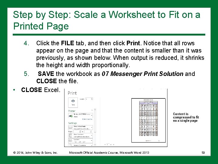
Step by Step: Scale a Worksheet to Fit on a Printed Page 4. Click the FILE tab, and then click Print. Notice that all rows appear on the page and that the content is smaller than it was previously, as shown below. When output is reduced, it shrinks the height and width proportionally. 5. SAVE the workbook as 07 Messenger Print Solution and CLOSE the file. • CLOSE Excel. © 2014, John Wiley & Sons, Inc. Microsoft Official Academic Course, Microsoft Word 2013 59

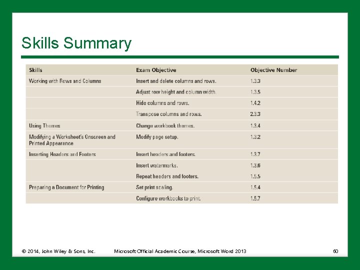
Skills Summary © 2014, John Wiley & Sons, Inc. Microsoft Official Academic Course, Microsoft Word 2013 60