Microsoft Azure prof dr Angelina Njegu Associate Professor

Microsoft Azure prof. dr Angelina Njeguš Associate Professor at Singidunum University anjegus@singidunum. ac. rs www. singidunum. ac. rs

Azure in education Did you know that educators, students, university researchers, and IT professionals at educational institutions have access to development tools and Azure services at no charge?

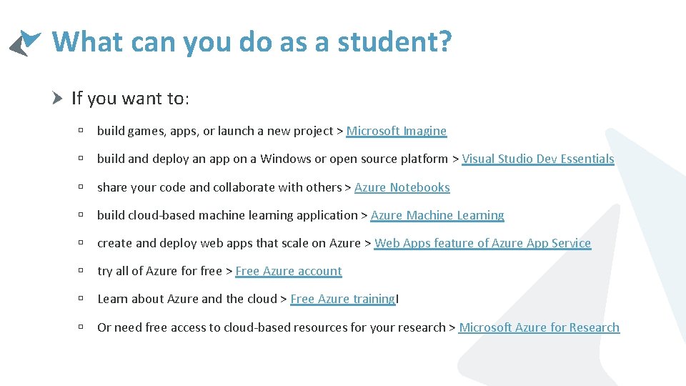
What can you do as a student? If you want to: ú build games, apps, or launch a new project > Microsoft Imagine ú build and deploy an app on a Windows or open source platform > Visual Studio Dev Essentials ú share your code and collaborate with others > Azure Notebooks ú build cloud-based machine learning application > Azure Machine Learning ú create and deploy web apps that scale on Azure > Web Apps feature of Azure App Service ú try all of Azure for free > Free Azure account ú Learn about Azure and the cloud > Free Azure training. I ú Or need free access to cloud-based resources for your research > Microsoft Azure for Research

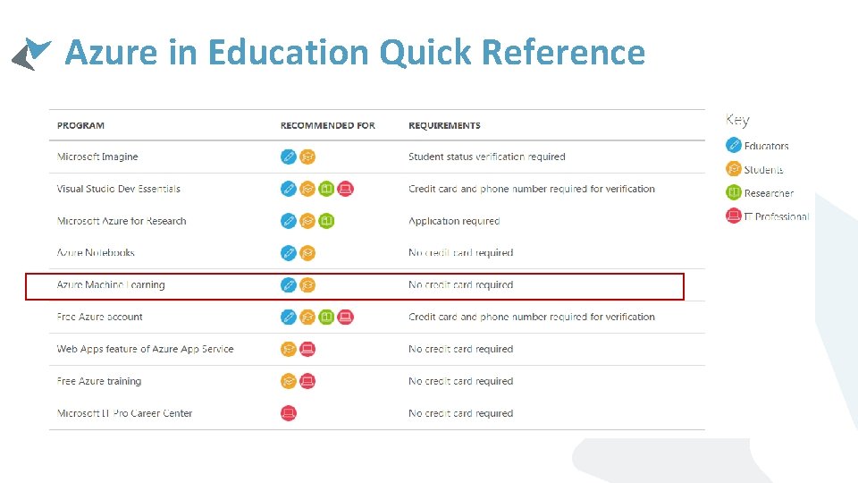
Azure in Education Quick Reference

Let’s start >

What is machine learning? Machine learning (ML) enables computers to learn from data and experiences and to act without being explicitly programmed. Azure Machine Learning is a cloud predictive analytics service that makes it possible to quickly create and deploy predictive models as analytics solutions. With ML Studio you can build Artificial Intelligence (AI) applications that intelligently sense, process, and act on information - augmenting human capabilities, increasing speed and efficiency, and helping organizations achieve more.

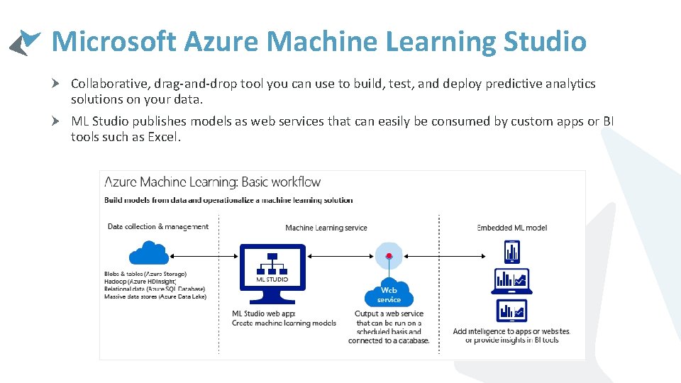
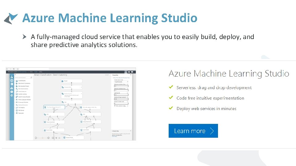
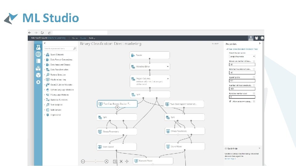
Microsoft Azure Machine Learning Studio Collaborative, drag-and-drop tool you can use to build, test, and deploy predictive analytics solutions on your data. ML Studio publishes models as web services that can easily be consumed by custom apps or BI tools such as Excel.

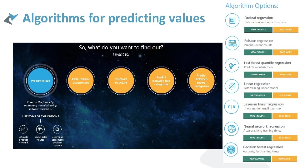
Algorithms for predicting values

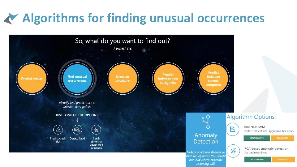
Algorithms for finding unusual occurrences

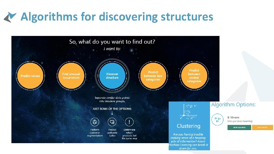
Algorithms for discovering structures

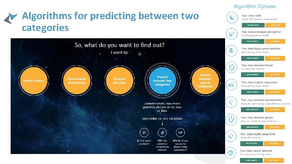
Algorithms for predicting between two categories

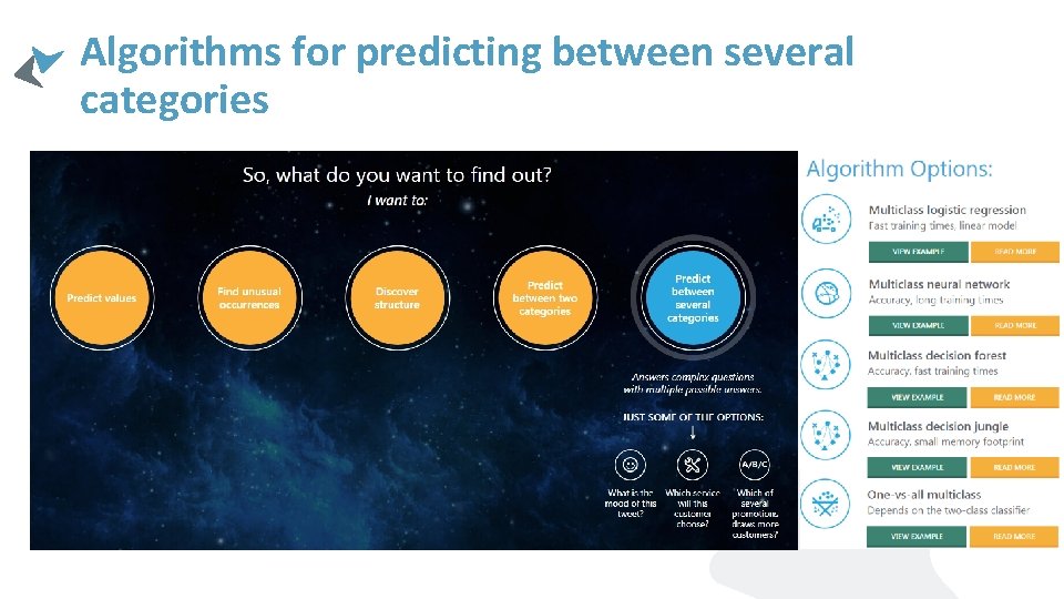
Algorithms for predicting between several categories

Azure Machine Learning Studio A fully-managed cloud service that enables you to easily build, deploy, and share predictive analytics solutions.

ML Studio

Five steps to create an experiment Before you start: ú Open Machine Learning Studio: https: //studio. azureml. net and Sign In. If you’ve signed into Machine Learning Studio before, click Sign In. Otherwise, click Sign up here and choose between free and paid options. Create a model ú Step 1: Get data ú Step 2: Prepare the data ú Step 3: Define features Train the model ú Step 4: Choose and apply a learning algorithm Score and test the model ú Step 5: Predict new automobile prices

Step 1: Get data There are several sample datasets included with Machine Learning Studio that you can use, or you can import data from many sources. For this example, we'll use the sample dataset, Automobile price data (Raw), that's included in your workspace. This dataset includes entries for various individual automobiles, including information such as make, model, technical specifications, and price.

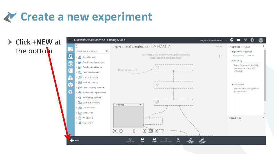
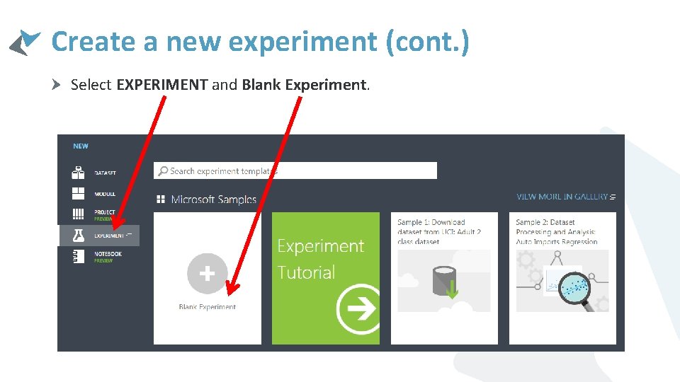
Create a new experiment Click +NEW at the bottom

Create a new experiment (cont. ) Select EXPERIMENT and Blank Experiment.

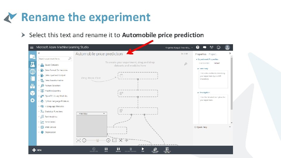
Rename the experiment Select this text and rename it to Automobile price prediction

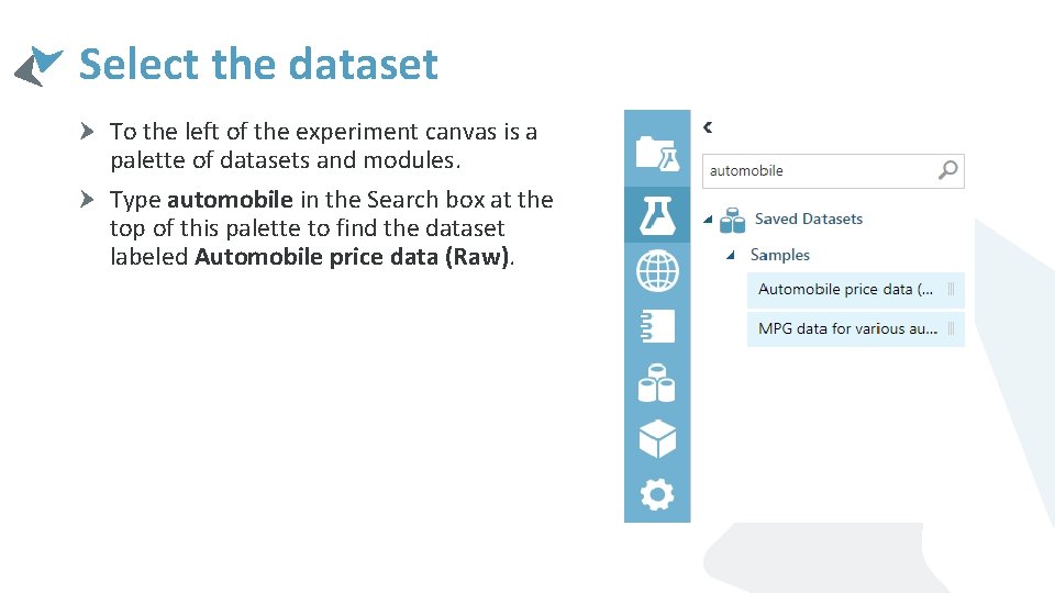
Select the dataset To the left of the experiment canvas is a palette of datasets and modules. Type automobile in the Search box at the top of this palette to find the dataset labeled Automobile price data (Raw).

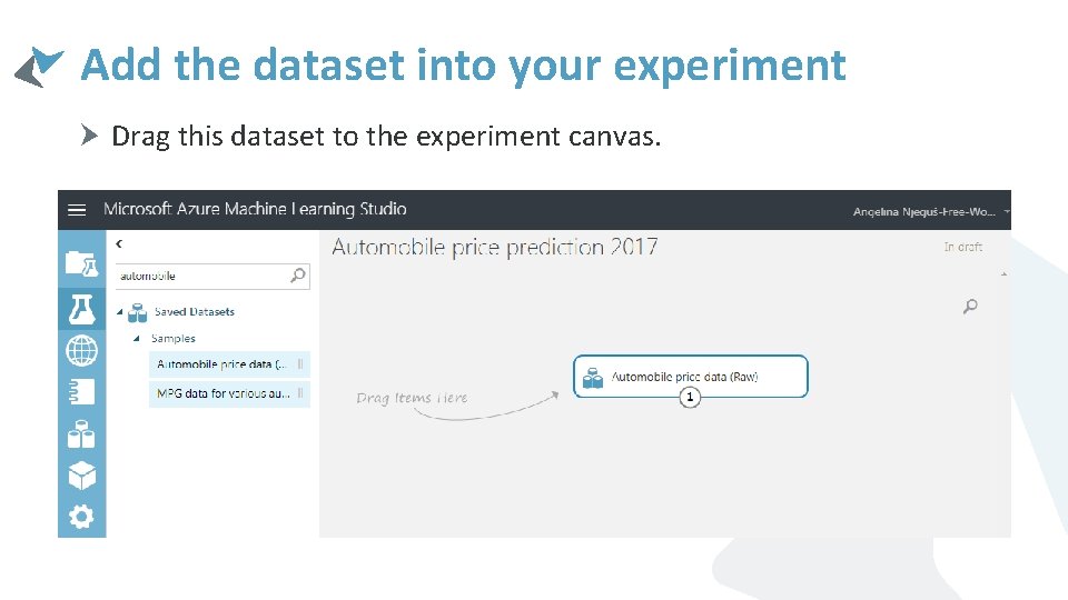
Add the dataset into your experiment Drag this dataset to the experiment canvas.

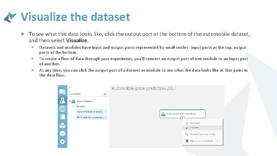
Visualize the dataset To see what this data looks like, click the output port at the bottom of the automobile dataset, and then select Visualize. ú ú ú Datasets and modules have input and output ports represented by small circles - input ports at the top, output ports at the bottom. To create a flow of data through your experiment, you'll connect an output port of one module to an input port of another. At any time, you can click the output port of a dataset or module to see what the data looks like at that point in the data flow.

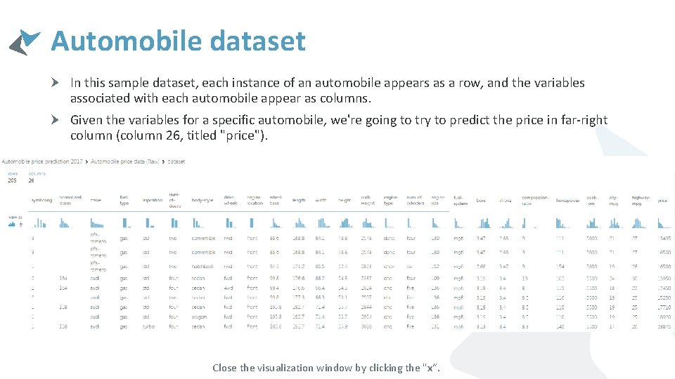
Automobile dataset In this sample dataset, each instance of an automobile appears as a row, and the variables associated with each automobile appear as columns. Given the variables for a specific automobile, we're going to try to predict the price in far-right column (column 26, titled "price"). Close the visualization window by clicking the "x“.

Step 2: Prepare the data A dataset usually requires some preprocessing before it can be analyzed. ú For example, you might have noticed the missing values present in the columns of various rows. ú These missing values need to be cleaned so the model can analyze the data correctly. ú In our case, we'll remove any rows that have missing values. The normalized-losses column has a large proportion of missing values, so we'll exclude that column from the model altogether. First we add a module that removes the normalized-losses column completely, and then we add another module that removes any row that has missing data.

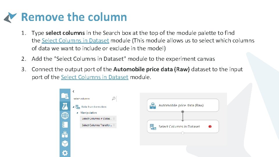
Remove the column 1. Type select columns in the Search box at the top of the module palette to find the Select Columns in Dataset module (This module allows us to select which columns of data we want to include or exclude in the model) 2. Add the "Select Columns in Dataset" module to the experiment canvas 3. Connect the output port of the Automobile price data (Raw) dataset to the input port of the Select Columns in Dataset module.

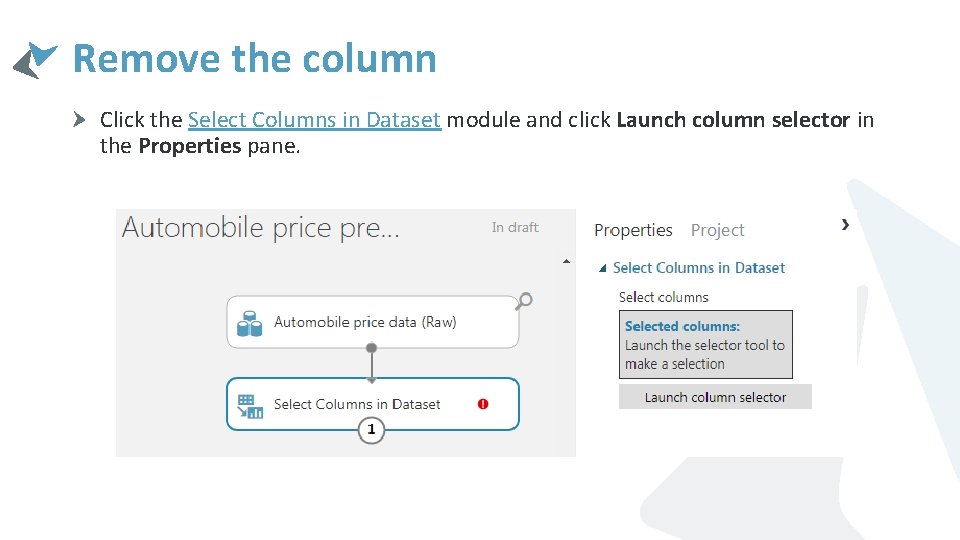
Remove the column Click the Select Columns in Dataset module and click Launch column selector in the Properties pane.

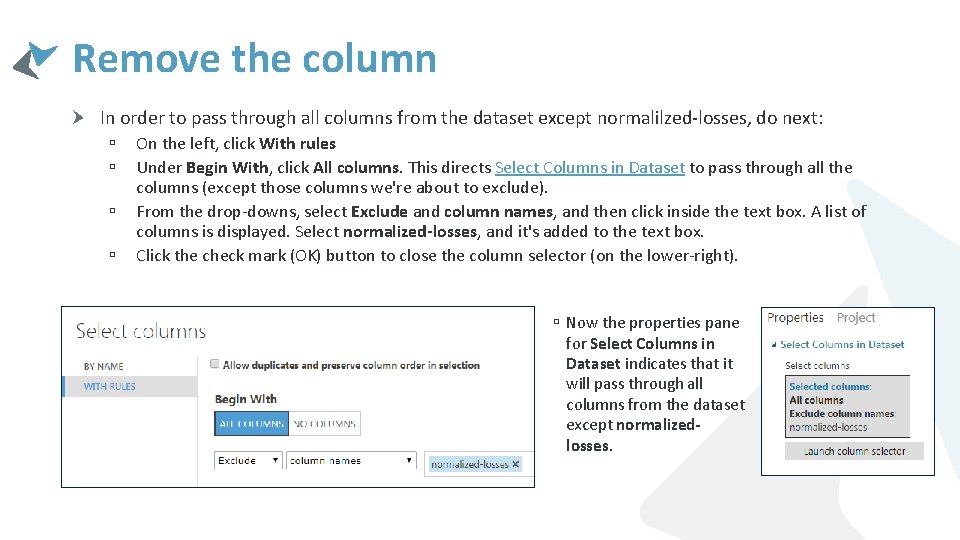
Remove the column In order to pass through all columns from the dataset except normalilzed-losses, do next: ú ú On the left, click With rules Under Begin With, click All columns. This directs Select Columns in Dataset to pass through all the columns (except those columns we're about to exclude). From the drop-downs, select Exclude and column names, and then click inside the text box. A list of columns is displayed. Select normalized-losses, and it's added to the text box. Click the check mark (OK) button to close the column selector (on the lower-right). ú Now the properties pane for Select Columns in Dataset indicates that it will pass through all columns from the dataset except normalizedlosses.

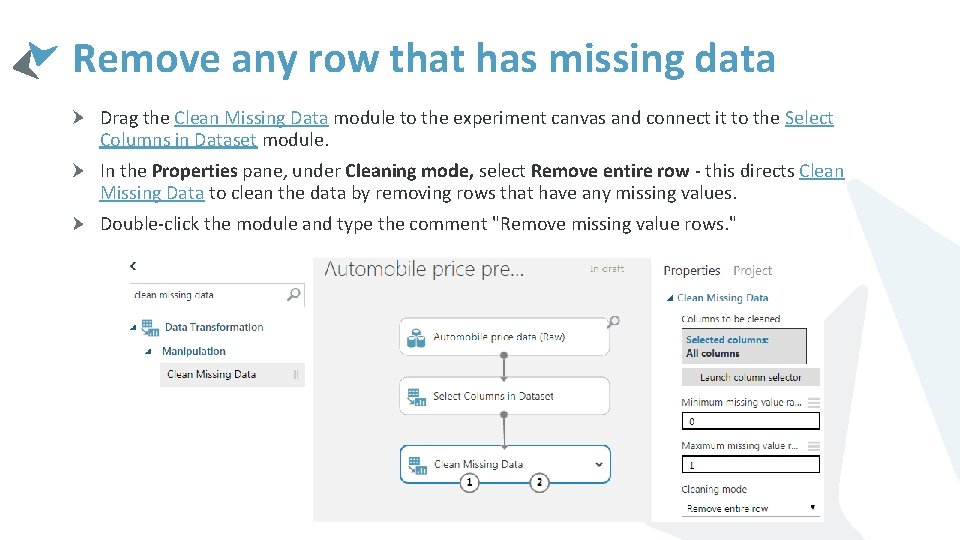
Remove any row that has missing data Drag the Clean Missing Data module to the experiment canvas and connect it to the Select Columns in Dataset module. In the Properties pane, under Cleaning mode, select Remove entire row - this directs Clean Missing Data to clean the data by removing rows that have any missing values. Double-click the module and type the comment "Remove missing value rows. "

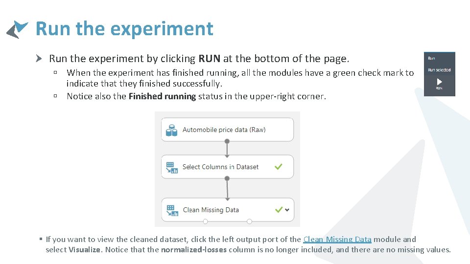
Run the experiment by clicking RUN at the bottom of the page. ú When the experiment has finished running, all the modules have a green check mark to indicate that they finished successfully. ú Notice also the Finished running status in the upper-right corner. § If you want to view the cleaned dataset, click the left output port of the Clean Missing Data module and select Visualize. Notice that the normalized-losses column is no longer included, and there are no missing values.

Step 3: Define features In dataset each row represents one automobile, and each column is a feature of that automobile. Finding a good set of features for creating a predictive model requires experimentation and knowledge about the problem you want to solve. ú Some features are better for predicting the target than others. ú Also, some features have a strong correlation with other features and can be removed. ú For example, city-mpg and highway-mpg are closely related so we can keep one and remove the other without significantly affecting the prediction. Let's build a model that uses a subset of the features in our dataset. You can come back later and select different features, run the experiment again, and see if you get better results.

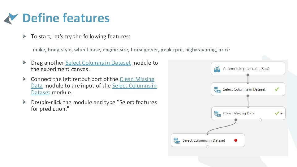
Define features To start, let's try the following features: make, body-style, wheel-base, engine-size, horsepower, peak-rpm, highway-mpg, price Drag another Select Columns in Dataset module to the experiment canvas. Connect the left output port of the Clean Missing Data module to the input of the Select Columns in Dataset module. Double-click the module and type "Select features for prediction. "

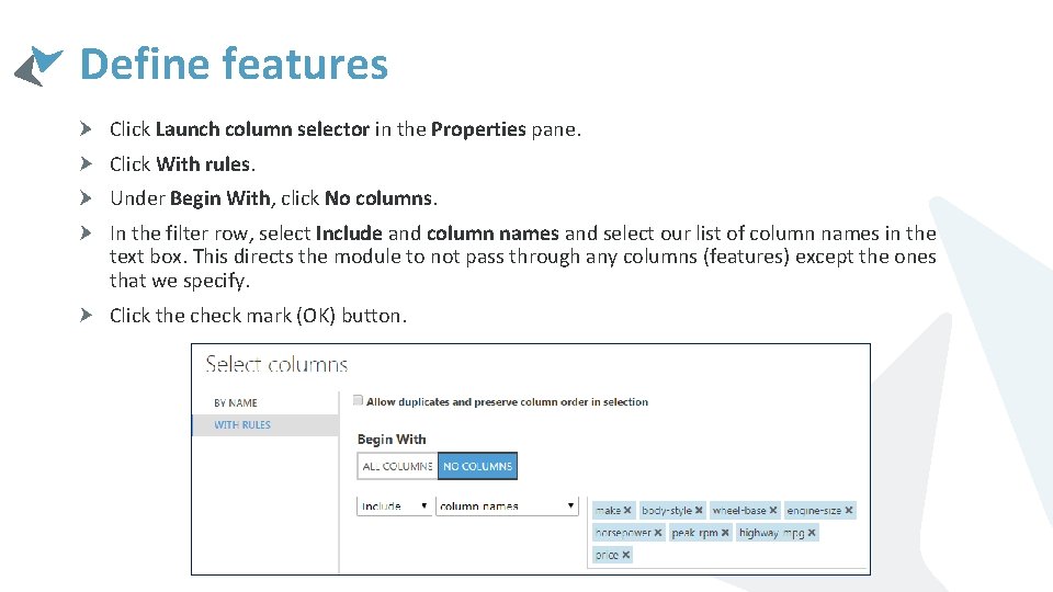
Define features Click Launch column selector in the Properties pane. Click With rules. Under Begin With, click No columns. In the filter row, select Include and column names and select our list of column names in the text box. This directs the module to not pass through any columns (features) except the ones that we specify. Click the check mark (OK) button.

Step 4: Choose and apply a learning algorithm Now that the data is ready, constructing a predictive model consists of training and testing. ú We'll use our data to train the model, and then we'll test the model to see how closely it's able to predict prices. Classification and regression are two types of supervised machine learning algorithms. ú Classification predicts an answer from a defined set of categories, such as a color (red, blue, or green). Regression is used to predict a number. Because we want to predict price, which is a number, we'll use a regression algorithm. For this example, we'll use a simple linear regression model.

Train and test the model We train the model by giving it a set of data that includes the price. The model scans the data and look for correlations between an automobile's features and its price. Then we'll test the model - we'll give it a set of features for automobiles we're familiar with and see how close the model comes to predicting the known price. We'll use our data for both training the model and testing it by splitting the data into separate training and testing datasets.

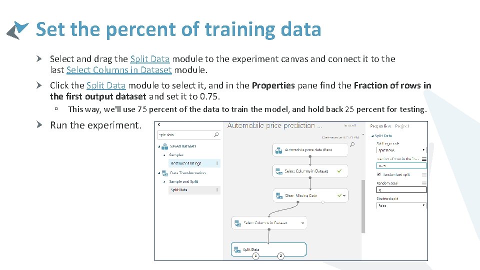
Set the percent of training data Select and drag the Split Data module to the experiment canvas and connect it to the last Select Columns in Dataset module. Click the Split Data module to select it, and in the Properties pane find the Fraction of rows in the first output dataset and set it to 0. 75. ú This way, we'll use 75 percent of the data to train the model, and hold back 25 percent for testing. Run the experiment.

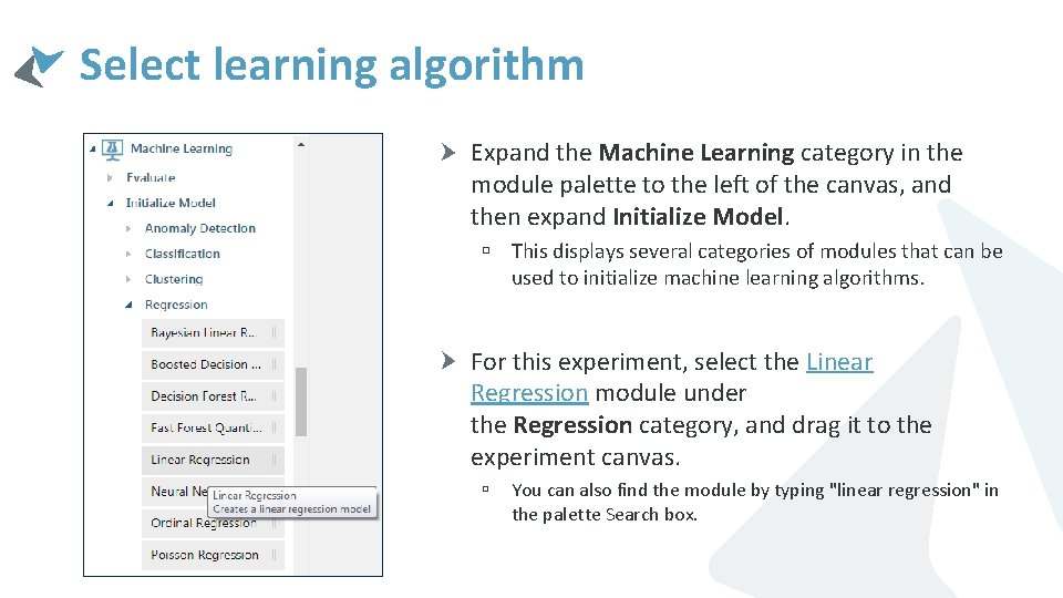
Select learning algorithm Expand the Machine Learning category in the module palette to the left of the canvas, and then expand Initialize Model. ú This displays several categories of modules that can be used to initialize machine learning algorithms. For this experiment, select the Linear Regression module under the Regression category, and drag it to the experiment canvas. ú You can also find the module by typing "linear regression" in the palette Search box.

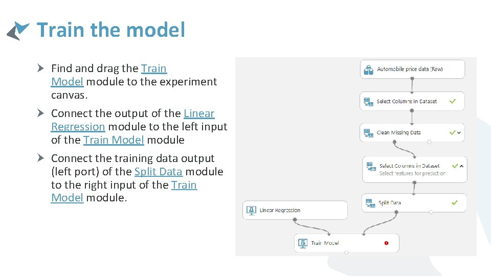
Train the model Find and drag the Train Model module to the experiment canvas. Connect the output of the Linear Regression module to the left input of the Train Model module Connect the training data output (left port) of the Split Data module to the right input of the Train Model module.

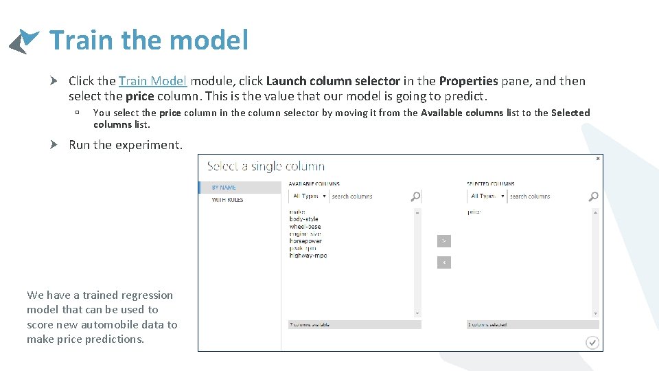
Train the model Click the Train Model module, click Launch column selector in the Properties pane, and then select the price column. This is the value that our model is going to predict. ú You select the price column in the column selector by moving it from the Available columns list to the Selected columns list. Run the experiment. We have a trained regression model that can be used to score new automobile data to make price predictions.

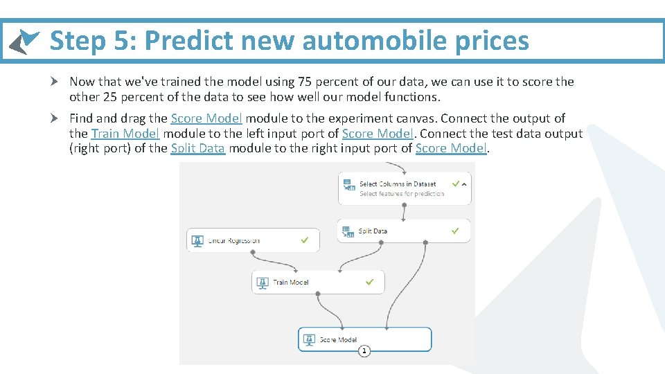
Step 5: Predict new automobile prices Now that we've trained the model using 75 percent of our data, we can use it to score the other 25 percent of the data to see how well our model functions. Find and drag the Score Model module to the experiment canvas. Connect the output of the Train Model module to the left input port of Score Model. Connect the test data output (right port) of the Split Data module to the right input port of Score Model.

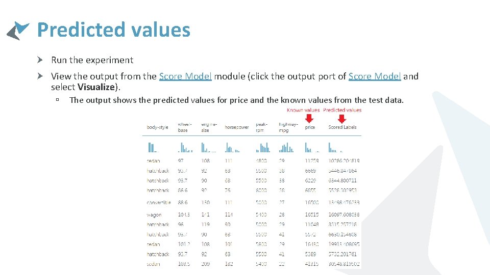
Predicted values Run the experiment View the output from the Score Model module (click the output port of Score Model and select Visualize). ú The output shows the predicted values for price and the known values from the test data.

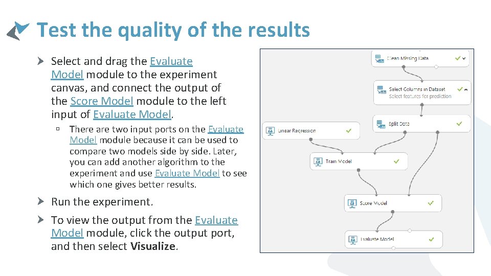
Test the quality of the results Select and drag the Evaluate Model module to the experiment canvas, and connect the output of the Score Model module to the left input of Evaluate Model. ú There are two input ports on the Evaluate Model module because it can be used to compare two models side by side. Later, you can add another algorithm to the experiment and use Evaluate Model to see which one gives better results. Run the experiment. To view the output from the Evaluate Model module, click the output port, and then select Visualize.

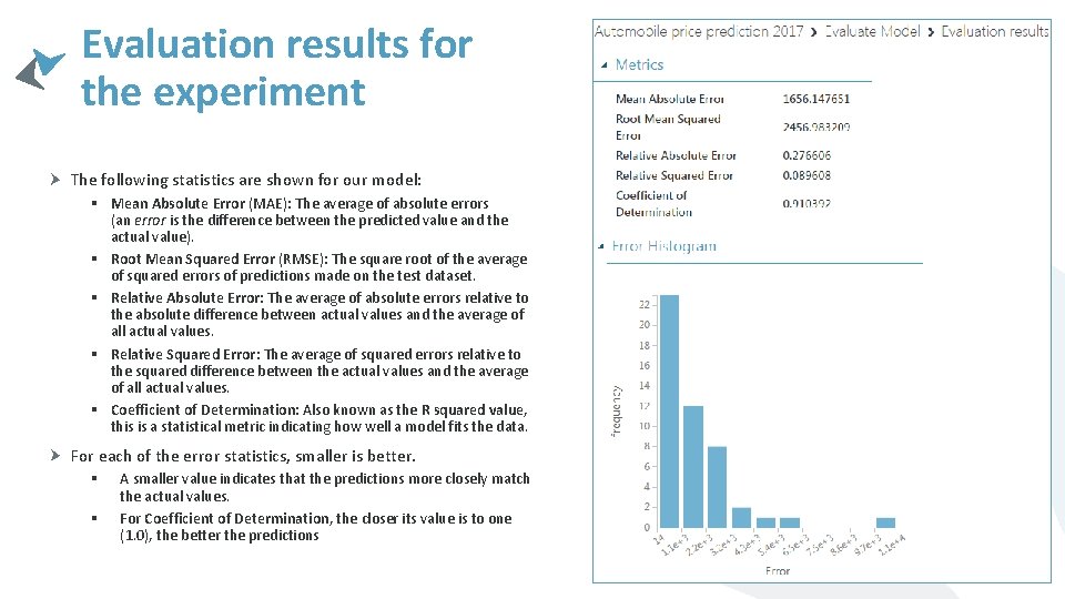
Evaluation results for the experiment The following statistics are shown for our model: § Mean Absolute Error (MAE): The average of absolute errors (an error is the difference between the predicted value and the actual value). § Root Mean Squared Error (RMSE): The square root of the average of squared errors of predictions made on the test dataset. § Relative Absolute Error: The average of absolute errors relative to the absolute difference between actual values and the average of all actual values. § Relative Squared Error: The average of squared errors relative to the squared difference between the actual values and the average of all actual values. § Coefficient of Determination: Also known as the R squared value, this is a statistical metric indicating how well a model fits the data. For each of the error statistics, smaller is better. § § A smaller value indicates that the predictions more closely match the actual values. For Coefficient of Determination, the closer its value is to one (1. 0), the better the predictions

Next steps Continue to improve the model and then deploy it as a predictive web service. ú Iterate to try to improve the model - For example: change the features for prediction. modify the properties of the Linear Regression algorithm try a different algorithm altogether. add multiple machine learning algorithms to experiment at one time and compare two of them by using the Evaluate Model module. For an example of how to compare multiple models in a single experiment, see Compare Regressors in the Cortana Intelligence Gallery. ú Deploy the model as a predictive web service - When you're satisfied with your model, you can deploy it as a web service to be used to predict automobile prices by using new data. For more details, see Deploy an Azure Machine Learning web service.

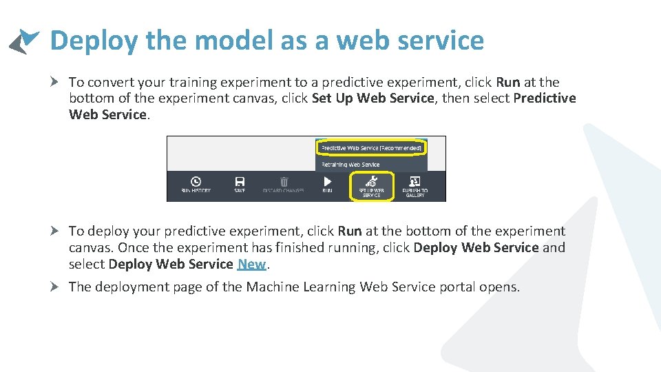
Deploy the model as a web service To convert your training experiment to a predictive experiment, click Run at the bottom of the experiment canvas, click Set Up Web Service, then select Predictive Web Service. To deploy your predictive experiment, click Run at the bottom of the experiment canvas. Once the experiment has finished running, click Deploy Web Service and select Deploy Web Service New. The deployment page of the Machine Learning Web Service portal opens.

Machine Learning Web Service portal Deploy Experiment Page Test your New web service ú To test your new web service, click Test web service under common tasks. On the Test page, you can test your web service as a Request-Response Service (RRS) or a Batch Execution service (BES). ú The RRS test page displays the inputs, outputs, and any global parameters that you have defined for the experiment. To test the web service, you can manually enter appropriate values for the inputs or supply a comma separated value (CSV) formatted file containing the test values. ú To test using RRS, from the list view mode, enter appropriate values for the inputs and click Test Request-Response. Your prediction results display in the output column to the left.