MICROARRAY DATA REPRESENTED by a N M matrix

MICROARRAY DATA REPRESENTED by a N × M matrix contains the gene expressions for the N genes of the jth tissue sample (j = 1, …, M). N = No. of genes (103 - 104) M = No. of tissue samples (10 - 102) STANDARD STATISTICAL METHODOLOGY APPROPRIATE FOR M >> N HERE N >> M

Microarray Data represented as N x M Matrix Sample 1 Sample 2 Expression Signature Gene 1 Gene 2 Expression Profile Gene N Sample M M columns (samples) ~ 102 N rows (genes) ~ 104

Two Clustering Problems: • Clustering of genes on basis of tissues: genes not independent • Clustering of tissues on basis of genes: latter is a nonstandard problem in cluster analysis (n << p)
 INFER CLASS LABELS z 1, …, zn of y 1,")
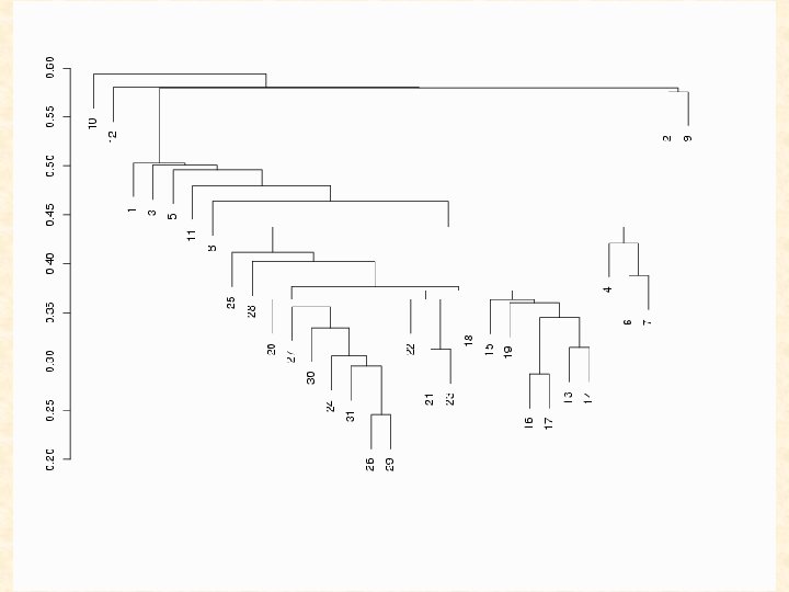
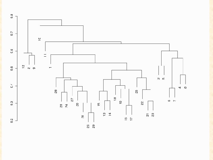
UNSUPERVISED CLASSIFICATION (CLUSTER ANALYSIS) INFER CLASS LABELS z 1, …, zn of y 1, …, yn Initially, hierarchical distance-based methods of cluster analysis were used to cluster the tissues and the genes Eisen, Spellman, Brown, & Botstein (1998, PNAS)

The notion of a cluster is not easy to define. There is a very large literature devoted to clustering when there is a metric known in advance; e. g. k-means. Usually, there is no a priori metric (or equivalently a user-defined distance matrix) for a cluster analysis. That is, the difficulty is that the shape of the clusters is not known until the clusters have been identified, and the clusters cannot be effectively identified unless the shapes are known.

In this case, one attractive feature of adopting mixture models with elliptically symmetric components such as the normal or t densities, is that the implied clustering is invariant under affine transformations of the data (that is, under operations relating to changes in location, scale, and rotation of the data). Thus the clustering process does not depend on irrelevant factors such as the units of measurement or the orientation of the clusters in space.

Hierarchical clustering methods for the analysis of gene expression data caught on like the hula hoop. I, for one, will be glad to see them fade. Gary Churchill (The Jackson Laboratory) Contribution to the discussion of the paper by Sebastiani, Gussoni, Kohane, and Ramoni. Statistical Science (2003) 18, 64 -69.
 clustering algorithms are largely heuristically motivated and there exist a number of")
Hierarchical (agglomerative) clustering algorithms are largely heuristically motivated and there exist a number of unresolved issues associated with their use, including how to determine the number of clusters. “in the absence of a well-grounded statistical model, it seems difficult to define what is meant by a ‘good’ clustering algorithm or the ‘right’ number of clusters. ” (Yeung et al. , 2001, Model-Based Clustering and Data Transformations for Gene Expression Data, Bioinformatics 17)
. On a resampling approach for tests on the number")
Mc. Lachlan and Khan (2004). On a resampling approach for tests on the number of clusters with mixture model-based clustering of the tissue samples. Special issue of the Journal of Multivariate Analysis 90 (2004) edited by Mark van der Laan and Sandrine Dudoit (UC Berkeley).

Attention is now turning towards a model-based approach to the analysis of microarray data For example: • Broet, Richarson, and Radvanyi (2002). Bayesian hierarchical model for identifying changes in gene expression from microarray experiments. Journal of Computational Biology 9 • Ghosh and Chinnaiyan (2002). Mixture modelling of gene expression data from microarray experiments. Bioinformatics 18 • Liu, Zhang, Palumbo, and Lawrence (2003). Bayesian clustering with variable and transformation selection. In Bayesian Statistics 7 • Pan, Lin, and Le, 2002, Model-based cluster analysis of microarray gene expression data. Genome Biology 3 • Yeung et al. , 2001, Model based clustering and data transformations for gene expression data, Bioinformatics 17

The notion of a cluster is not easy to define. There is a very large literature devoted to clustering when there is a metric known in advance; e. g. k-means. Usually, there is no a priori metric (or equivalently a user-defined distance matrix) for a cluster analysis. That is, the difficulty is that the shape of the clusters is not known until the clusters have been identified, and the clusters cannot be effectively identified unless the shapes are known.

In this case, one attractive feature of adopting mixture models with elliptically symmetric components such as the normal or t densities, is that the implied clustering is invariant under affine transformations of the data (that is, under operations relating to changes in location, scale, and rotation of the data). Thus the clustering process does not depend on irrelevant factors such as the units of measurement or the orientation of the clusters in space.
, Finite Mixture Models.")
http: //www. maths. uq. edu. au/~g Mc. Lachlan and Peel (2000), Finite Mixture Models. Wiley.


Mixture Software: EMMIX for UNIX Mc. Lachlan, Peel, Adams, and Basford http: //www. maths. uq. edu. au/~gjm/emmix. html

Basic Definition We let Y 1, …. Yn denote a random sample of size n where Yj is a p-dimensional random vector with probability density function f (yj) where the f i(yj) are densities and the pi are nonnegative quantities that sum to one.

Mixture distributions are applied to data with two main purposes in mind: • To provide an appealing semiparametric framework in which to model unknown distributional shapes, as an alternative to, say, the kernel density method. • To use the mixture model to provide a modelbased clustering. (In both situations, there is the question of how many components to include in the mixture. )

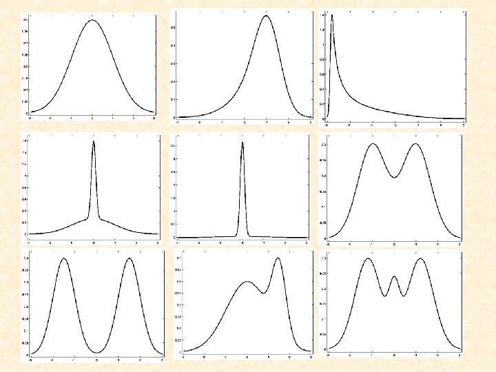
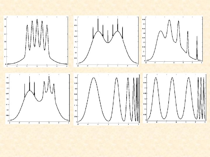
Shapes of Some Univariate Normal Mixtures Consider where denotes the univariate normal density with mean m and variance s 2.

D=1 D=3 D=2 D=4 Figure 1: Plot of a mixture density of two univariate normal components in equal proportions with common variance s 2=1

D=1 D=3 D=2 D=4 Figure 2: Plot of a mixture density of two univariate normal components in proportions 0. 75 and 0. 25 with common variance

Normal Mixtures • Computationally convenient for multivariate data • Provide an arbitrarily accurate estimate of the underlying density with g sufficiently large • Provide a probabilistic clustering of the data into g clusters - outright clustering by assigning a data point to the component to which it has the greatest posterior probability of belonging

Synthetic Data Set 1

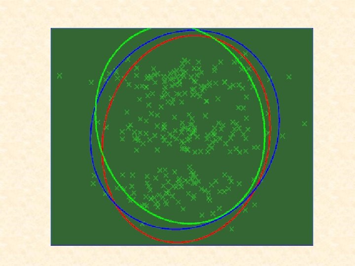
Synthetic Data Set 2

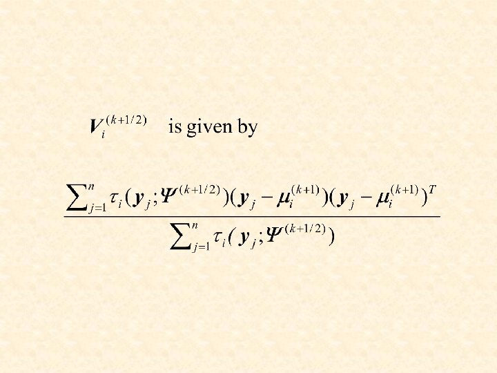
y p 1 True Values 0. 333 0. 294 p 2 p 3 m 1 m 2 m 3 S 1 0. 333 0. 337 0. 333 0. 370 (0 – 2)T (-1 0) T (-0. 154 – 1. 961) T (0 0) T (0. 360 0. 115) T (0 2) T (1 0) T (-0. 004 2. 027) T S 1 Initial Values Estimates by EM

Figure 7
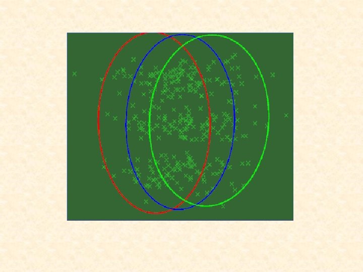

Figure 8

MIXTURE OF g NORMAL COMPONENTS where constant MAHALANOBIS DISTANCE EUCLIDEAN DISTANCE

MIXTURE OF g NORMAL COMPONENTS k-means SPHERICAL CLUSTERS

Equal spherical covariance matrices

With a mixture model-based approach to clustering, an observation is assigned outright to the ith cluster if its density in the ith component of the mixture distribution (weighted by the prior probability of that component) is greater than in the other (g-1) components.

Figure 7: Contours of the fitted component densities on the 2 nd & 3 rd variates for the blue crab data set.

Estimation of Mixture Distributions It was the publication of the seminal paper of Dempster, Laird, and Rubin (1977) on the EM algorithm that greatly stimulated interest in the use of finite mixture distributions to model heterogeneous data. Mc. Lachlan and Krishnan (1997, Wiley)

• If need be, the normal mixture model can be made less sensitive to outlying observations by using t component densities. • With this t mixture model-based approach, the normal distribution for each component in the mixture is embedded in a wider class of elliptically symmetric distributions with an additional parameter called the degrees of freedom.

The advantage of the t mixture model is that, although the number of outliers needed for breakdown is almost the same as with the normal mixture model, the outliers have to be much larger.

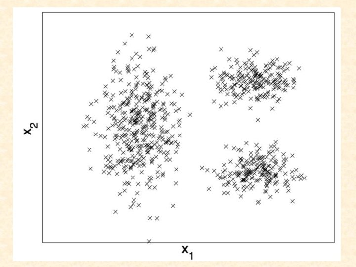
In exploring high-dimensional data sets for group structure, it is typical to rely on principal component analysis.

Two Groups in Two Dimensions. All cluster information would be lost by collapsing to the first principal component. The principal ellipses of the two groups are shown as solid curves.

Mixtures of Factor Analyzers A normal mixture model without restrictions on the component-covariance matrices may be viewed as too general for many situations in practice, in particular, with high dimensional data. One approach for reducing the number of parameters is to work in a lower dimensional space by using principal components; another is to use mixtures of factor analyzers (Ghahramani & Hinton, 1997).

Mixtures of Factor Analyzers Principal components or a single-factor analysis model provides only a global linear model. A global nonlinear approach by postulating a mixture of linear submodels

Bi is a p x q matrix and Di is a diagonal matrix.

Single-Factor Analysis Model
 independently of the errors ej, which are iid")
The Uj are iid N(O, Iq) independently of the errors ej, which are iid as N(O, D), where D is a diagonal matrix

Conditional on ith component membership of the mixture, where Ui 1, . . . , Uin are independent, identically distibuted (iid) N(O, Iq), independently of the eij, which are iid N(O, Di), where Di is a diagonal matrix (i = 1, . . . , g).

An infinity of choices for Bi for model still holds if Bi is replaced by Bi. Ci where Ci is an orthogonal matrix. Choose Ci so that is diagonal Number of free parameters is then

Reduction in the number of parameters is then We can fit the mixture of factor analyzers model using an alternating ECM algorithm.

1 st cycle: declare the missing data to be the component-indicator vectors. Update the estimates of and 2 nd cycle: declare the missing data to be also the factors. Update the estimates of and

M-step on 1 st cycle: for i = 1, . . . , g.

M step on 2 nd cycle: where
 -1= Di – 1 -")
Work in q-dim space: (Bi. T + Di ) -1= Di – 1 - Di -1 Bi (Iq + Bi. TDi -1 Bi) -1 Bi. TDi -1, |Bi. T+D i| = | Di | / |Iq -Bi. T(Bi. T+Di) -1 Bi|.

where

With EM: where

To avoid potential computational problems with small-sized clusters, we impose the constraint

j

Number of Components in a Mixture Model Testing for the number of components, g, in a mixture is an important but very difficult problem which has not been completely resolved.

Order of a Mixture Model A mixture density with g components might be empirically indistinguishable from one with either fewer than g components or more than g components. It is therefore sensible in practice to approach the question of the number of components in a mixture model in terms of an assessment of the smallest number of components in the mixture compatible with the data.

Likelihood Ratio Test Statistic An obvious way of approaching the problem of testing for the smallest value of the number of components in a mixture model is to use the LRTS, -2 logl. Suppose we wish to test the null hypothesis, versus for some g 1>g 0.
. Then the")
We let denote the MLE of calculated under Hi , (i=0, 1). Then the evidence against H 0 will be strong if l is sufficiently small, or equivalently, if -2 logl is sufficiently large, where
 proposed a resampling approach to the assessment of")
Bootstrapping the LRTS Mc. Lachlan (1987) proposed a resampling approach to the assessment of the P-value of the LRTS in testing for a specified value of g 0.
 of Schwarz (1978) is given by")
Bayesian Information Criterion The Bayesian information criterion (BIC) of Schwarz (1978) is given by as the penalized log likelihood to be maximized in model selection, including the present situation for the number of components g in a mixture model.
 Clest (Dudoit and Fridlyand, 2002)")
Gap statistic (Tibshirani et al. , 2001) Clest (Dudoit and Fridlyand, 2002)

PROVIDES A MODEL-BASED APPROACH TO CLUSTERING Mc. Lachlan, Bean, and Peel, 2002, A Mixture Model-Based Approach to the Clustering of Microarray Expression Data, Bioinformatics 18, 413 -422 http: //www. bioinformatics. oupjournals. org/cgi/screenpdf/18/3/ 413. pdf
 M = 62 (40")
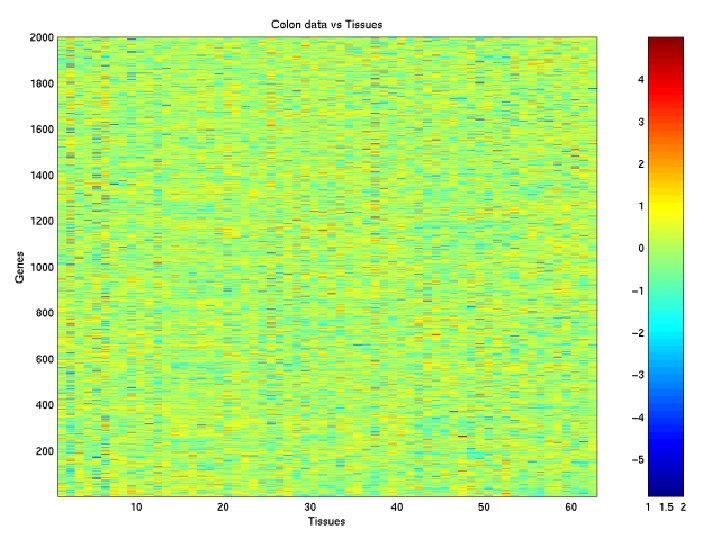
Example: Microarray Data Colon Data of Alon et al. (1999) M = 62 (40 tumours; 22 normals) tissue samples of N = 2, 000 genes in a 2, 000 62 matrix.

Mixture of 2 normal components

Mixture of 2 t components

The t distribution does not have substantially better breakdown behavior than the normal (Tyler, 1994). The advantage of the t mixture model is that, although the number of outliers needed for breakdown is almost the same as with the normal mixture model, the outliers have to be much larger. This point is made more precise in Hennig (2002) who has provided an excellent account of breakdown points for ML estimation of location -scale mixtures with a fixed number of components g. Of course as explained in Hennig (2002), mixture models can be made more robust by allowing the number of components g to grow with the number of outliers.

For Normal mixtures breakdown begins with an additional point at about 15. 2. For a mixture of t 3 -distributions, the outlier must lie at about 800, t 1 -mixtures need the outlier at about , and a Normal mixture with additional noise component breaks down with an additional point at
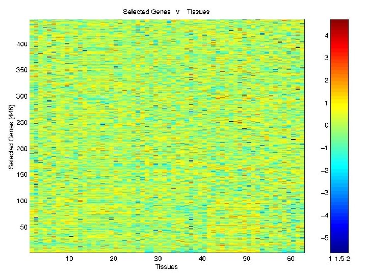

Clustering of COLON Data Genes using EMMIX-GENE

Grouping for Colon Data 1 6 2 7 11 16 3 8 12 17 4 9 13 18 5 10 14 19 15 20

Clustering of COLON Data Tissues using EMMIX-GENE

Grouping for Colon Data 1 6 2 7 11 16 3 8 12 17 4 9 13 18 5 10 14 19 15 20

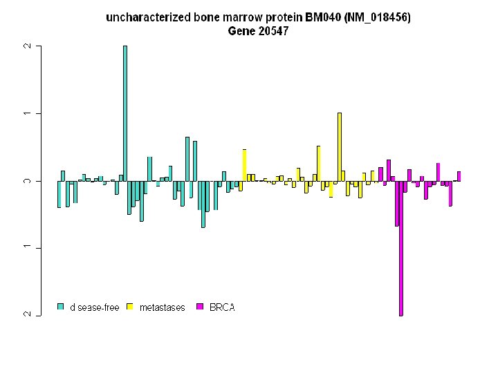
Heat Map Displaying the Reduced Set of 4, 869 Genes on the 98 Breast Cancer Tumours

Insert heat map of 1867 genes Heat Map of Top 1867 Genes

1 2 3 4 5 6 7 8 9 10 11 16 12 17 13 18 14 19 15 20

21 22 23 24 25 26 27 28 29 30 31 36 32 37 33 38 34 39 35 40

i 1 mi Ui 146 112. 98 i 11 mi 66 Ui 25. 72 i mi 21 44 Ui 13. 77 i mi 31 53 Ui 9. 84 2 93 74. 95 12 38 25. 45 22 30 13. 28 32 36 8. 95 3 61 46. 08 13 28 25. 00 23 25 13. 10 33 36 8. 89 4 55 35. 20 14 53 21. 33 24 67 13. 01 34 38 8. 86 5 43 30. 40 15 47 18. 14 25 12 12. 04 35 44 8. 02 6 92 29. 29 16 23 18. 00 26 58 12. 03 36 56 7. 43 7 71 28. 77 17 27 17. 62 27 27 11. 74 37 46 7. 21 8 20 28. 76 18 45 17. 51 28 64 11. 61 38 19 6. 14 9 23 28. 44 19 80 17. 28 29 38 11. 38 39 29 4. 64 10 23 27. 73 20 55 13. 79 30 21 10. 72 40 35 2. 44 where i = group number mi = number in group i Ui = -2 log λi

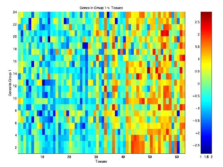
Heat Map of Genes in Group G 1

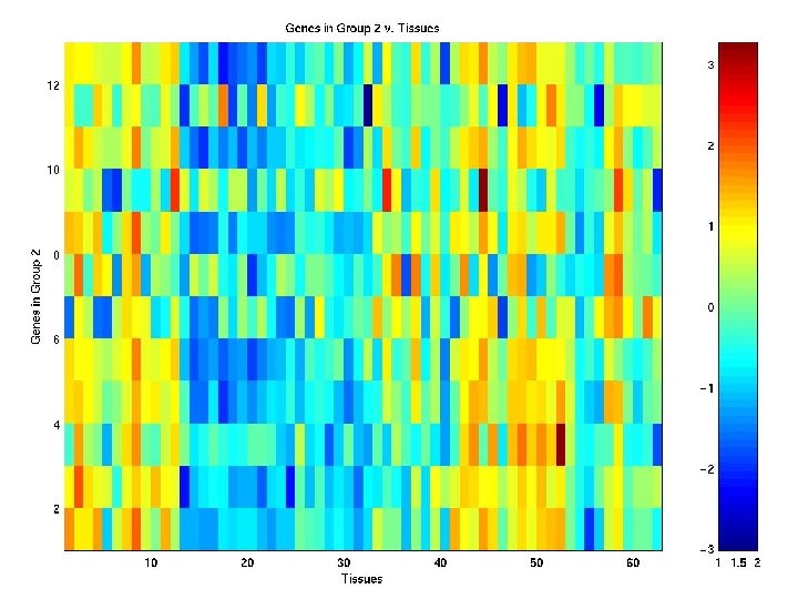
Heat Map of Genes in Group G 2

Heat Map of Genes in Group G 3
")
Clustering of gene expression profiles • Longitudinal (with or without replication, for example time-course) • Cross-sectional data EMMIX-WIRE EM-based MIXture analysis With Random Effects A Mixture Model with Random-Effects Components for Clustering Correlated Gene-Expression Profiles. S. K. Ng, G. J. Mc. Lachlan, K. Wang, L. Ben-Tovim Jones, S-W. Ng.

Clustering of Correlated Gene Profiles

Clustering of gene expression profiles • Longitudinal (with or without replication, for example time course) • Cross-section data
, with")
N(mh, Bh), with
th row")
Yeast Cell Cycle X is an 18 x 2 matrix with the (l+1)th row (l= 0, …, 17) Yeast data is from Spellman (1998); 18 rows represent the 18 α-factor (pheromone) synchronization where the yeast cells were sampled at 7 minute intervals for 119 minutes. ω is the period of the cell cycle and ξ is the phase offset, estimated using least squares to be ω=53 and ξ =0.

Clustering Results for Spellman Yeast Cell Cycle Data
 Our clustering (b) Muro clustering")
Plots of First versus Second Principal Components (a) Our clustering (b) Muro clustering

A Mixture Model with Random-Effects Components for Clustering Correlated Gene-Expression Profiles. S. K. Ng, G. J. Mc. Lachlan, K. Wang, L. Ben-Tovim Jones, S-W. Ng.
- Slides: 103