Micha Suchanek Advanced Statistical Methods Scientific method Observation

Michał Suchanek Advanced Statistical Methods

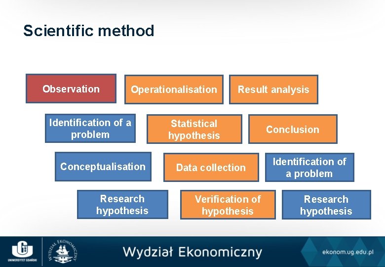
Scientific method Observation Operationalisation Identification of a problem Conceptualisation Research hypothesis Result analysis Statistical hypothesis Data collection Verification of hypothesis Conclusion Identification of a problem Research hypothesis

A brief reminder • constants, • variables; • population, • sample.

Variables • qualitative • quantitative: – discrete, – continuous,

Measurement • the process of assigning numbers to traits • Stevens scale (level of measurement): – – nominal, ordinal, interval, ratio scale.

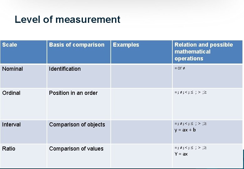
Level of measurement Scale Basis of comparison Examples Relation and possible mathematical operations Nominal Identification = or ≠ Ordinal Position in an order = ; ≠ ; < ; ≤ ; > ; ≥ Interval Comparison of objects = ; ≠ ; < ; ≤ ; > ; ≥ Ratio Comparison of values = ; ≠ ; < ; ≤ ; > ; ≥ y = ax + b Y = ax

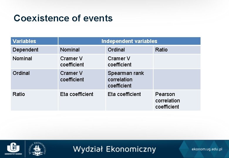
Coexistence of events Variables Independent variables Dependent Nominal Ordinal Nominal Cramer V coefficient Ordinal Cramer V coefficient Spearman rank correlation coefficient Ratio Eta coefficient Ratio Pearson correlation coefficient

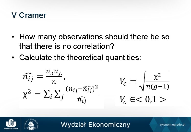
V Cramer • How many observations should there be so that there is no correlation? • Calculate theoretical quantities:

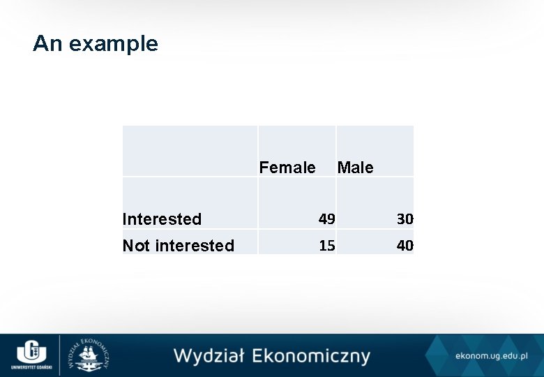
An example Female Male Interested 49 30 Not interested 15 40

ANOVA (analysis of variance) • used to determine if there are differences in ratio values between nominal groups • Ho : µ 1 = µ 2 = µ 3 = … = µk ; • HA : at least one group is significantly different from the others

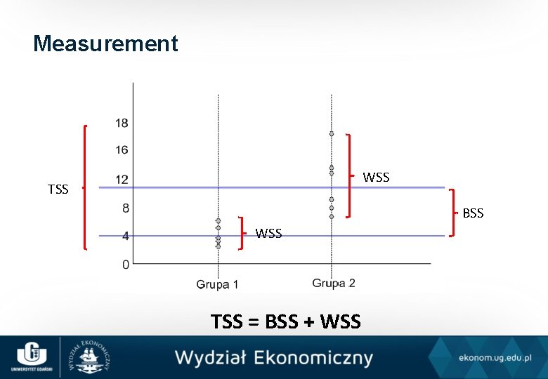
Measurement WSS TSS BSS WSS TSS = BSS + WSS

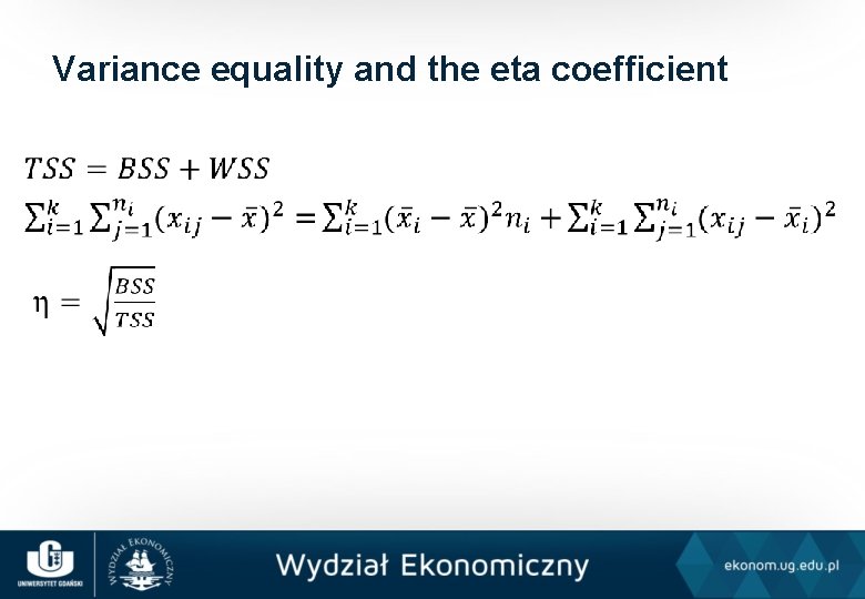
Variance equality and the eta coefficient

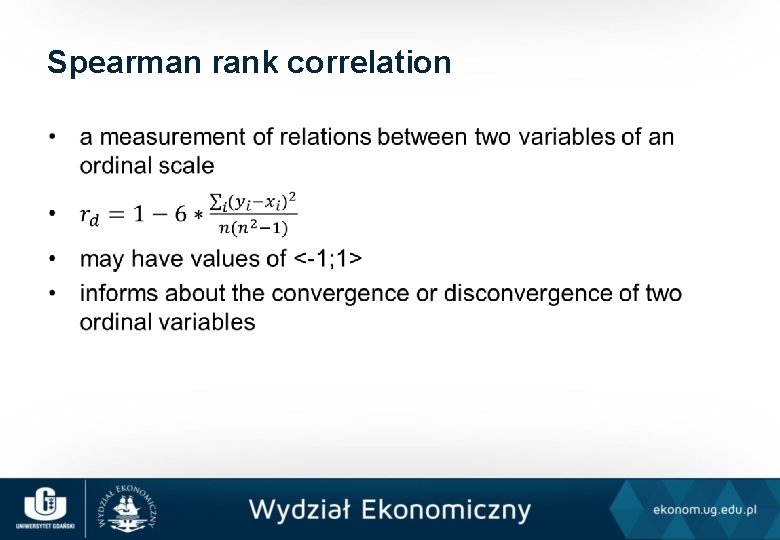
Spearman rank correlation •

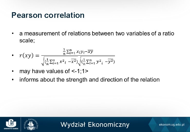
Pearson correlation •

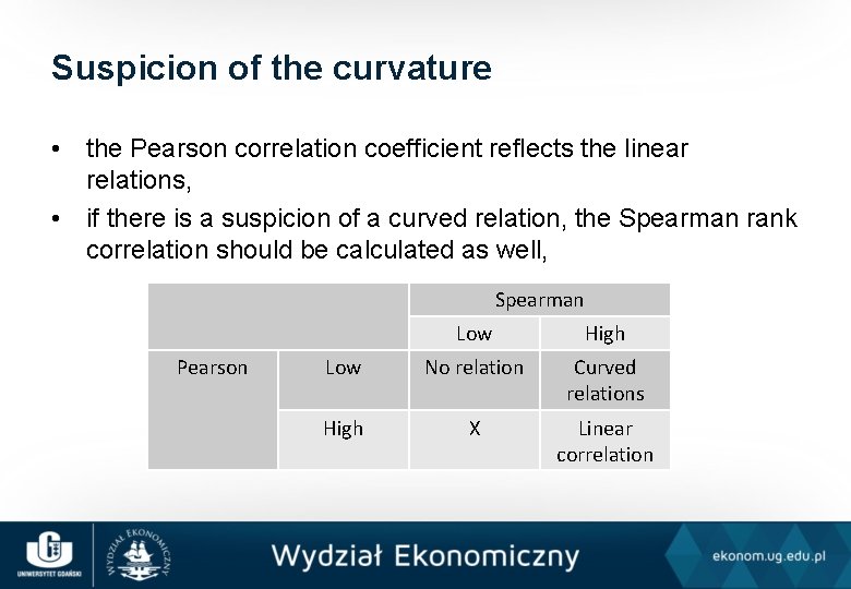
Suspicion of the curvature • the Pearson correlation coefficient reflects the linear relations, • if there is a suspicion of a curved relation, the Spearman rank correlation should be calculated as well, Spearman Pearson Low High Low No relation Curved relations High X Linear correlation

Spurious correlations • tylervigen. com

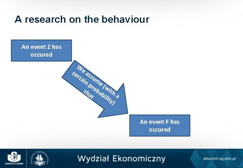
A research on the behaviour An event Z has occured W ce e as rta su in me pr (w th oba ith at bil a ity ) An event F has occured

An indicator • an indicator of the event F is an event Z, which, if it is observed, allows us to assume that the event F has occured as well

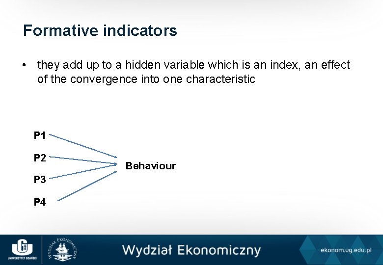
Formative indicators • they add up to a hidden variable which is an index, an effect of the convergence into one characteristic P 1 P 2 P 3 P 4 Behaviour

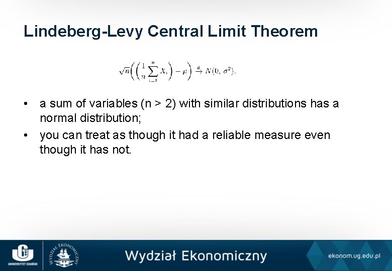
Lindeberg-Levy Central Limit Theorem • a sum of variables (n > 2) with similar distributions has a normal distribution; • you can treat as though it had a reliable measure even though it has not.

The defense and the construction of variable • the defense of the variable is twofold: – merits-related, – statistical, • the collective variable may be a result of a simple construction (e. g. a sum): • Likert scaling: – sum = Pos. 1+Pos. 2+…+Pos. k – weighted sum = w 1 Pos. 1+w 2 Pos. 2+…+wk. Pos. k

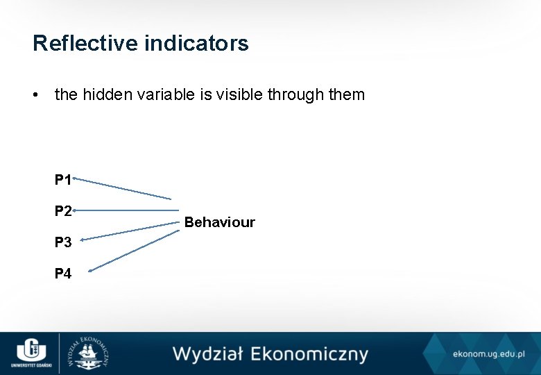
Reflective indicators • the hidden variable is visible through them P 1 P 2 P 3 P 4 Behaviour

The basic assumptions • the indicators have the same cause, therefore they have to be correlated, • if the indicators work the opposite way they should be rescaled, • the basis for the pertinent construction of the summary scale is for the variance of the sum to be different than the sum of variances.

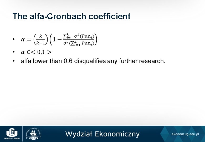
The alfa-Cronbach coefficient •

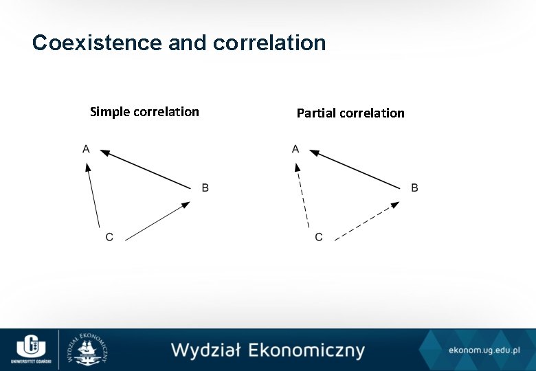
Coexistence and correlation Simple correlation Partial correlation

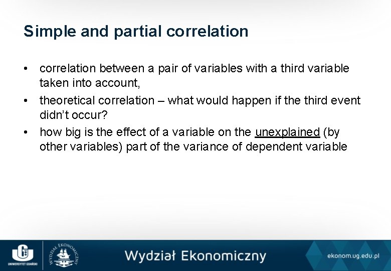
Simple and partial correlation • correlation between a pair of variables with a third variable taken into account, • theoretical correlation – what would happen if the third event didn’t occur? • how big is the effect of a variable on the unexplained (by other variables) part of the variance of dependent variable

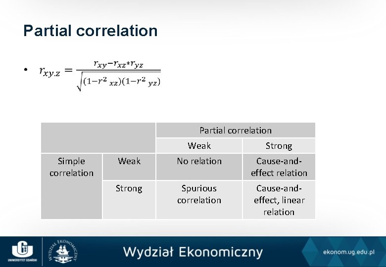
Partial correlation • Partial correlation Simple correlation Weak Strong Weak No relation Cause-andeffect relation Strong Spurious correlation Cause-andeffect, linear relation

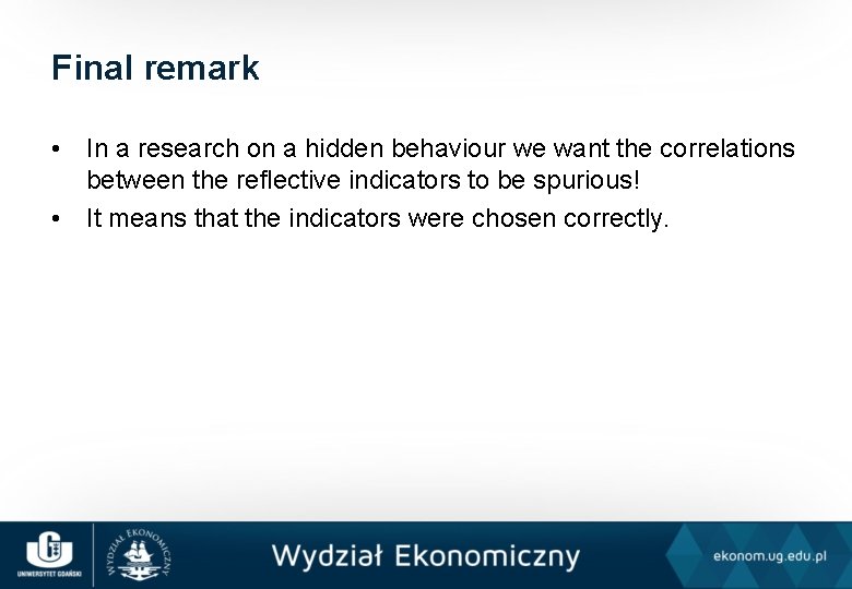
Final remark • In a research on a hidden behaviour we want the correlations between the reflective indicators to be spurious! • It means that the indicators were chosen correctly.

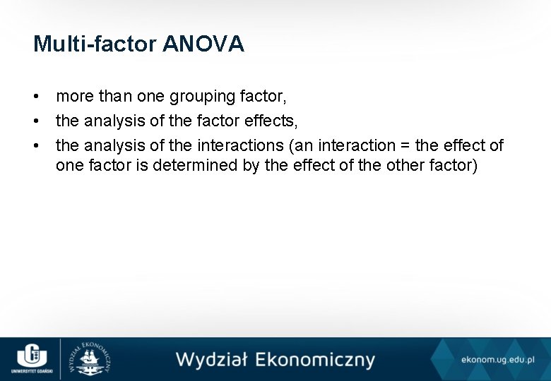
Multi-factor ANOVA • more than one grouping factor, • the analysis of the factor effects, • the analysis of the interactions (an interaction = the effect of one factor is determined by the effect of the other factor)

Underlying assumptions • random sampling, • independent observations, • normal distributions of the dependent variable within each group, but… (Box, 1953), • homoscedacity of the distributions within the groups.

Homoscedacity tests • Hartley (strongly relies on normality, requires even groups), • C Cochrane (strongly relies on normality, requires even groups), • Bartlett (strongly relies on normality), • Levene.

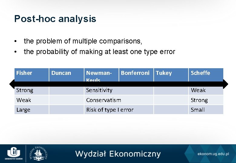
Post-hoc analysis • the problem of multiple comparisons, • the probability of making at least one type error Fisher Duncan Newman. Keuls Bonferroni Tukey Scheffe Strong Sensitivity Weak Conservatism Strong Large Risk of type I error Small

Covariance analysis (ANCOVA) • includes additional covariates (continuous variables) in the ANOVA, • a mix between the analysis of variance and regression

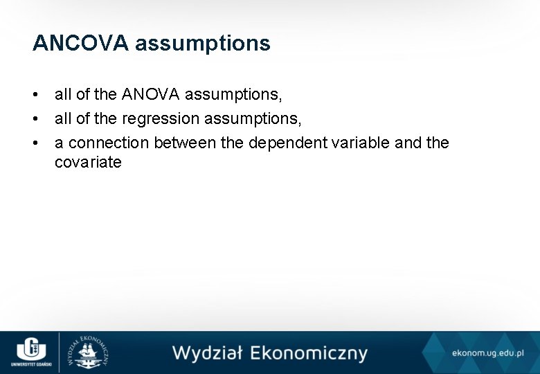
ANCOVA assumptions • all of the ANOVA assumptions, • all of the regression assumptions, • a connection between the dependent variable and the covariate

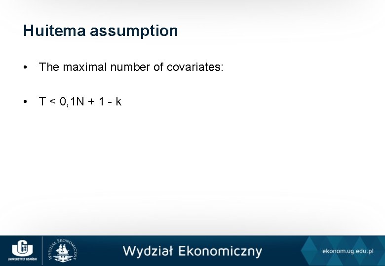
Huitema assumption • The maximal number of covariates: • T < 0, 1 N + 1 - k

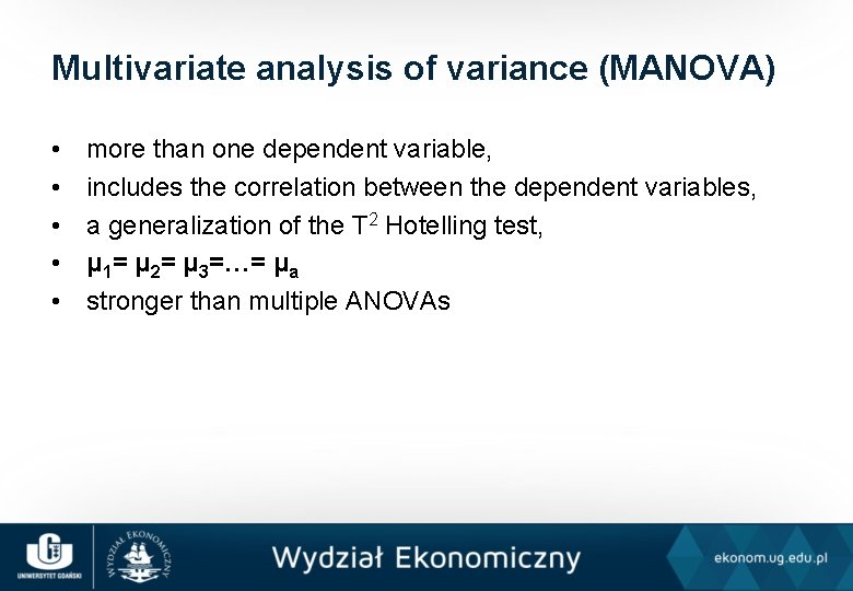
Multivariate analysis of variance (MANOVA) • • • more than one dependent variable, includes the correlation between the dependent variables, a generalization of the T 2 Hotelling test, μ 1= μ 2= μ 3=…= μa stronger than multiple ANOVAs

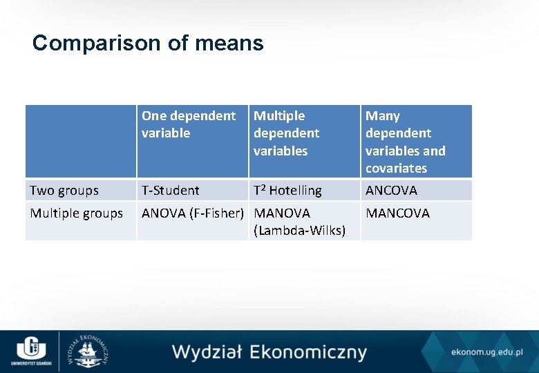
Comparison of means One dependent variable Multiple dependent variables Many dependent variables and covariates Two groups T-Student T 2 Hotelling ANCOVA Multiple groups ANOVA (F-Fisher) MANOVA (Lambda-Wilks) MANCOVA

MANOVA – the statistics • • Wilks’ Lambda, Pillai’s Trace – the strongest and most resilient, Lawley-Hotelling’s Trace, Roy’s largest root.

MANOVA – assumptions • independent observations, • the same variance-covariance matrix for all the populations – variance tests (similar as for ANOVA) and covariance M Box test, • multivariate normal distribution, • no outliers.

Principal Component Analysis (PCA) • • reduction of dimensions, analysis of the structure, verification of the connections, orthogonal transformation of variables into new, independent variables (not correlated)

Factor loadings • show the correlation between the factors and their components, • show the relative importance of collection of items

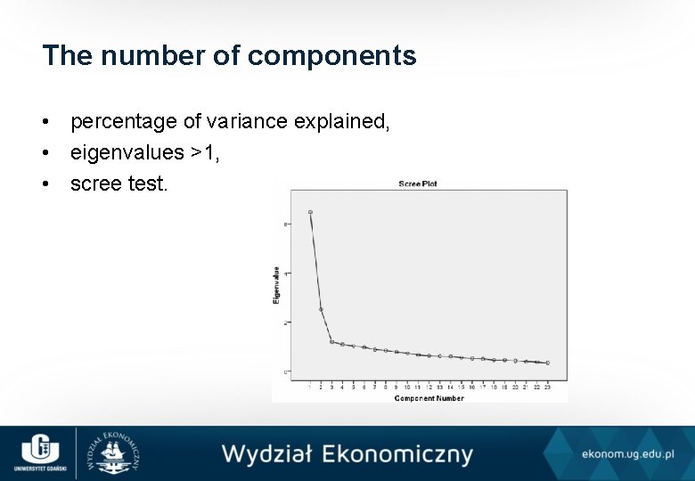
The number of components • percentage of variance explained, • eigenvalues >1, • scree test.

Assumptions • • theoretically at least ordinal scale variables, dependent and correlated variables, normality (only for significance testing), number of observations – at least 50, more like 100 (some sources: 5 observations per variable), • outliers, • missing data.

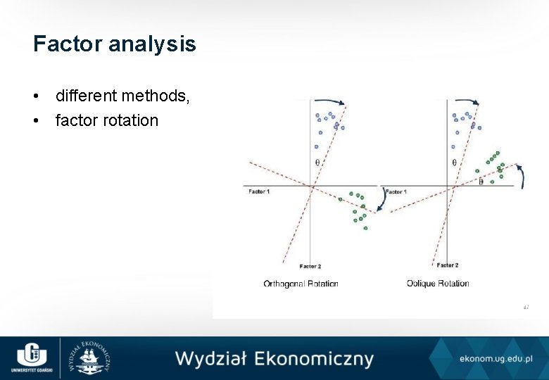
Factor analysis • different methods, • factor rotation

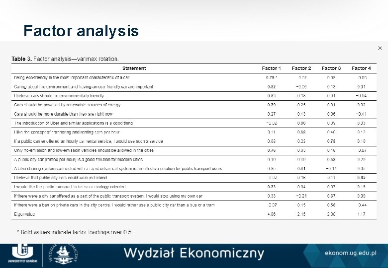
Factor analysis

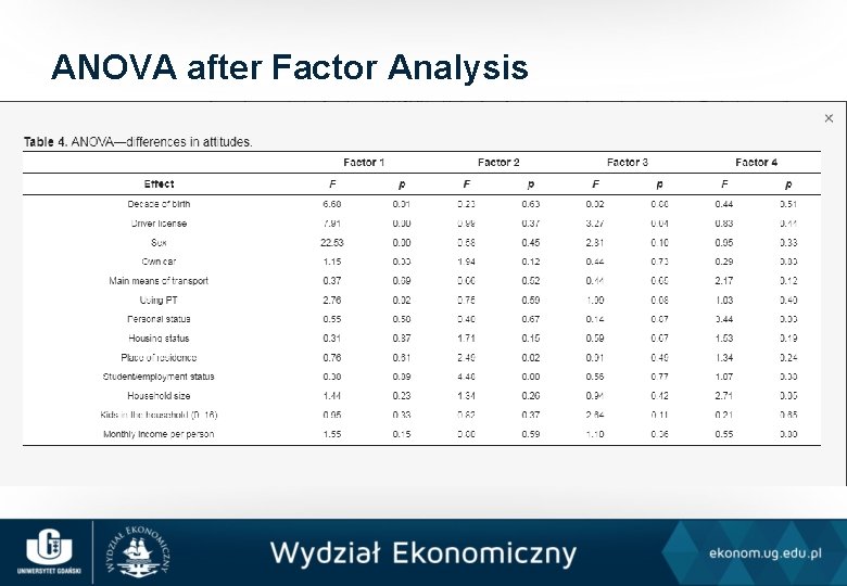
ANOVA after Factor Analysis

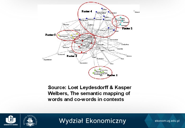
Source: Loet Leydesdorff & Kasper Welbers, The semantic mapping of words and co-words in contexts

Survival analysis • Procedures in which time at which an event happens is the measured variables • an event – change in the value of the variable, • survival time – period between the entry and the time of the event (T), • Censored observations

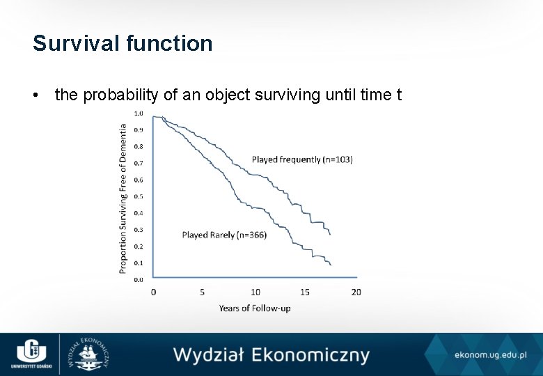
Survival function • the probability of an object surviving until time t

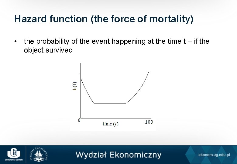
Hazard function (the force of mortality) • the probability of the event happening at the time t – if the object survived

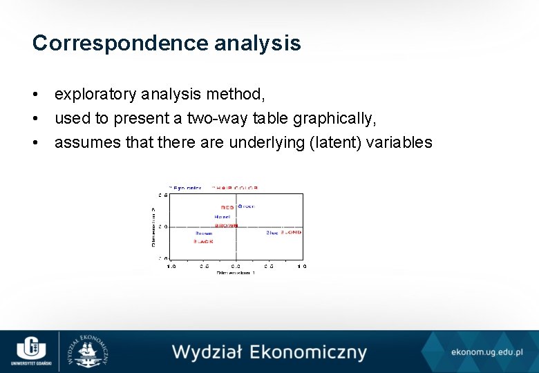
Correspondence analysis • exploratory analysis method, • used to present a two-way table graphically, • assumes that there are underlying (latent) variables

Log-linear analysis • The analysis of relations within the qualitative data • The method for the assessment of intensity between two or more groups of variables

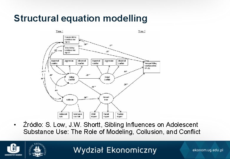
Structural equation modelling • Źródło: S. Low, J. W. Shortt, Sibling Influences on Adolescent Substance Use: The Role of Modeling, Collusion, and Conflict

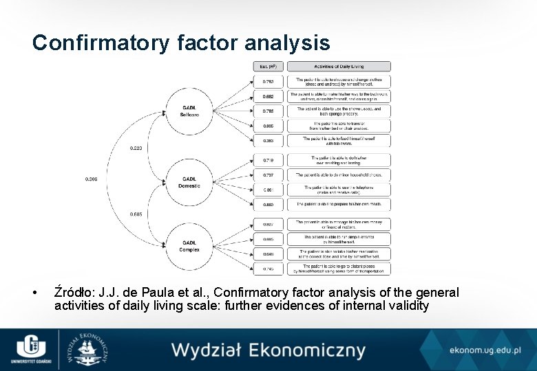
Confirmatory factor analysis • Źródło: J. J. de Paula et al. , Confirmatory factor analysis of the general activities of daily living scale: further evidences of internal validity

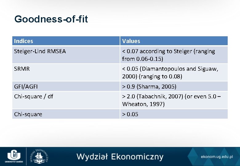
Goodness-of-fit Indices Values Steiger-Lind RMSEA < 0. 07 according to Steiger (ranging from 0. 06 -0. 15) SRMR < 0. 05 (Diamantopoulos and Siguaw, 2000) (ranging to 0. 08) GFI/AGFI > 0. 9 (Sharma, 2005) Chi-square / df > 2. 0 (Tabachnik, 2007) (or even 5. 0 – Wheaton, 1997) Chi-square > 0. 05