METU Department of Computer Eng Ceng 302 Introduction

METU Department of Computer Eng Ceng 302 Introduction to DBMS Indexing Structures for Files by Pinar Senkul resources: mostly froom Elmasri, Navathe and other books

Chapter Outline Types of Single-level Ordered Indexes Primary Indexes Clustering Indexes Secondary Indexes Multilevel Indexes Dynamic Multilevel Indexes Using B-Trees B+-Trees Indexes on Multiple Keys and

Indexes as Access Paths A single-level index is an auxiliary file that makes it more efficient to search for a record in the data file. The index is usually specified on one field of the file (although it could be specified on several fields) One form of an index is a file of entries <field value, pointer to record>, which is ordered by field value The index is called an access path on the field.

Indexes as Access Paths The index file usually occupies considerably less disk blocks than the data file because its entries are much smaller A binary search on the index yields a pointer to the file record Indexes can also be characterized as dense or sparse. A dense index has an index entry for every search key value (and hence every record) in the data file. A sparse (or nondense) index, on the other hand, has index entries for only some of the search values

Example: Given the following data file: EMPLOYEE(NAME, SSN, ADDRESS, JOB, SAL, . . . ) Suppose that: record size R=150 bytes block size B=512 bytes r=30000 records Then, we get: blocking factor Bfr= B div R= 512 div 150= 3 records/block number of file blocks b= (r/Bfr)= (30000/3)= 10000 blocks For an index on the SSN field, assume the field size VSSN=9 bytes, assume the record pointer size PR=7 bytes. Then: index entry size RI=(VSSN+ PR)=(9+7)=16 bytes index blocking factor Bfr. I= B div RI= 512 div 16= 32 entries/block number of index blocks b= (r/ Bfr. I)= (30000/32)= 938 blocks binary search needs log 2 b. I= log 2938= 10 block accesses This is compared to an average linear search cost of: (b/2)= 10000/2= 5000 block accesses If the file records are ordered, the binary search cost would be: log 2 b= log 210000= 14 block accesses

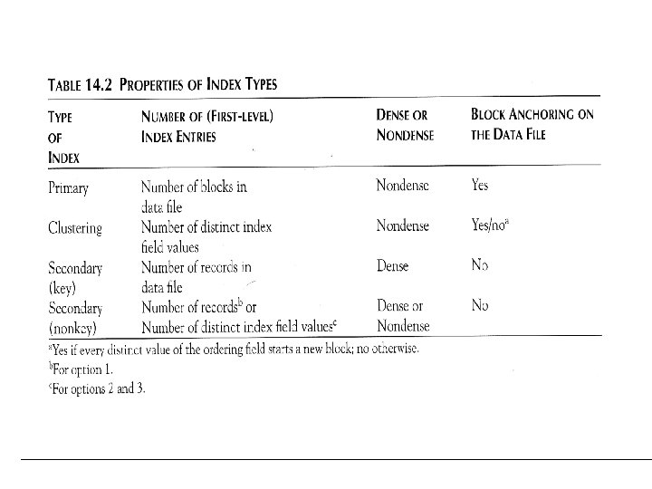
Types of Single-Level Indexes Primary Index Clustering Index Secondary Index

Primary Indexes Defined on an ordered data file The data file is ordered on a key field Includes one index entry for each block in the data file; the index entry has the key field value for the first record in the block, which is called the block anchor A similar scheme can use the last record in a block. A primary index is a nondense (sparse) index, since it includes an entry for each disk block of the data file and the keys of its anchor record rather than for every search value.

Primary index on the ordering key field of the file

Example: Given the following data file: EMPLOYEE(NAME, SSN, ADDRESS, JOB, SAL, . . . ) Suppose that: record size R=150 bytes block size B=512 bytes r=30000 records Then, we get: blocking factor Bfr= B div R= 512 div 150= 3 records/block number of file blocks b= (r/Bfr)= (30000/3)= 10000 blocks For a primary ndex on the SSN field, assume the field size VSSN=9 bytes, assume the record pointer size PR=7 bytes. Then: index entry size RI=(VSSN+ PR)=(9+7)=16 bytes index blocking factor Bfr. I= B div RI= 512 div 16= 32 entries/block number of index blocks bi= (b/ Bfr. I)= (10000/32)= 313 blocks binary search needs log 2 bi= log 2 313= 9 block accesses One more disk access to get the record itself. Total 10 block accesses

Clustering Index Defined on an ordered data file The data file is ordered on a non-key field unlike primary index, which requires that the ordering field of the data file have a distinct value for each record. Includes one index entry for each distinct value of the field; the index entry points to the first data block that contains records with that field value. It is another example of nondense index where Insertion and Deletion is relatively straightforward with a clustering index.

A clustering index on the DEPTNUMBER ordering nonkey field of an EMPLOYEE file.

Clustering index with a separate block cluster for each group of records that share the same value for the clustering field.

Example: Given the following data file: EMPLOYEE(NAME, SSN, ADDRESS, JOB, SAL, . . . ) Suppose that: record size R=150 bytes block size B=512 bytes r=30000 records Then, we get: blocking factor Bfr= B div R= 512 div 150= 3 records/block number of file blocks b= (r/Bfr)= (30000/3)= 10000 blocks For a clustering index on the DNO field, assume the field size VSSN=9 bytes, assume the record pointer size PR=7 bytes. Then: index entry size RI=(VSSN+ PR)=(9+7)=16 bytes index blocking factor Bfr. I= B div RI= 512 div 16= 32 entries/block Assume that there are 50 distinct department numbers. number of index blocks bi= (50/ Bfr. I)= (50/32)= 2 blocks binary search needs log 2 2= 1 block access To access to the record we must do at least 1 more block access. (More may be needed to follow the pointers

Secondary Index A secondary index provides a secondary means of accessing a file for which some primary access already exists. The secondary index may be on a field which is a candidate key and has a unique value in every record, or a nonkey with duplicate values. The index is an ordered file with two fields. The first field is of the same data type as some nonordering field of the data file that is an indexing field. The second field is either a block pointer or a record pointer. There can be many secondary indexes (and hence, indexing fields) for the same file. Includes one entry for each record in the data file; hence, it is a dense index

A dense secondary index (with block pointers) on a nonordering key field of a file.

A secondary index (with recored pointers) on a nonkey field implemented using one level of indirection so that index entries are of fixed length and have unique field values.

Multi-Level Indexes Because a single-level index is an ordered file, we can create a primary index to the index itself ; in this case, the original index file is called the first-level index and the index to the index is called the second-level index. We can repeat the process, creating a third, fourth, . . . , top level until all entries of the top level fit in one disk block A multi-level index can be created for any type of first-level index (primary, secondary, clustering) as long as the firstlevel index consists of more than one disk block

A two-level primary index resembling ISAM (Indexed Sequential Access Method) organization

Example: Suppose that: record size R=100 bytes block size B=1024 bytes r=30000 records Then, we get: blocking factor Bfr= B div R= 1024 div 100= 10 records/block number of file blocks b= (r/Bfr)= (30000/10)= 3000 blocks For a secondary index on nonordering key field, assume the field size VSSN=9 bytes, assume the record pointer size PR=6 bytes. Then: index entry size RI=(VSSN+ PR)=(9+6)=15 bytes index blocking factor Bfr. I= B div RI= 1024 div 15= 68 entries/block number of index blocks bi= (r/ Bfr. I)= (30000/68)= 442 blocks binary search needs log 2 bi= log 2 442= 9 block accesses If we convert this structure into multi-level index: We calculated that Bfri = 68 number of index blocks at second level b 2 = (bi / Bfri) = (442 / 68) = 7 blocks number of index blocks at third level b 3 = (b 2 / Bfri) = (7 / 68) = 1 blocks To access to a record : 3 block access (for each level) + 1 (for record itself ) = 4

Multi-Level Indexes Such a multi-level index is a form of search tree; however, insertion and deletion of new index entries is a severe problem because every level of the index is an ordered file.

A node in a search tree with pointers to subtrees below it.

A search tree of order p = 3.

Dynamic Multilevel Indexes Using B-Trees and B+-Trees Because of the insertion and deletion problem, most multilevel indexes use B-tree or B+-tree data structures, which leave space in each tree node (disk block) to allow for new index entries These data structures are variations of search trees that allow efficient insertion and deletion of new search values. In B-Tree and B+-Tree data structures, each node corresponds to a disk block Each node is kept between half-full and completely full (Analysis show that, the nodes are 69% full when the number of values in the tree stabilizes. )

Dynamic Multilevel Indexes Using B-Trees and B+-Trees An insertion into a node that is not full is quite efficient; if a node is full the insertion causes a split into two nodes Splitting may propagate to other tree levels A deletion is quite efficient if a node does not become less than half full If a deletion causes a node to become less than half full, it must be merged with neighboring nodes

Difference between B-tree and B+-tree In a B-tree, pointers to data records exist at all levels of the tree In a B+-tree, all pointers to data records exists at the leaf-level nodes A B+-tree can have less levels (or higher capacity of search values) than the corresponding B-tree

B-tree structures. (a) A node in a B-tree with q – 1 search values. (b) A B-tree of order p = 3. The values were inserted in the order 8, 5, 1, 7, 3, 12, 9, 6.

B-Trees Assume that in a B-tree, V=9 bytes - search field B= 512 bytes – block size Pr = 7 bytes – data pointer P = 6 bytes – tree pointer Each node can have at most q tree pointers, (q-1) data pointers and (q-1) search key field values. Therefore: (q*P)+((q-1)*(Pr+V) ≤ B ---> q = 23

B-Trees Assume that in a B-tree with q=23 nodes are 69% full. 23*0. 69=16 pointers at each node approximately. root: 1 node 15 entries 16 pointers level 1: 16 nodes 240 entries 256 pointers level 2: 256 nodes 3840 entries 4096 pointers level 3: 4096 nodes 61440 entries

The nodes of a B+-tree. (a) Internal node of a B+-tree with q – 1 search values. (b) Leaf node of a B+-tree with q – 1 search values and q – 1 data pointers.

B+ Trees Assume that in a B+ tree, V=9 bytes - search field B= 512 bytes – block size Pr = 7 bytes – data pointer P = 6 bytes – tree pointer Each internal node can have at most q tree pointers and (q-1) search key field values. Therefore: (q*P)+((q-1)*V) ≤ B ---> q = 34 Each leaf node can have at most p data pointers, p search key field values and a next pointer. (p * (Pr+V) + P) ≤ B ---> p = 31

B+ Trees Assume that in a B+ tree with q=34 and p=31, nodes are 69% full. 34*0. 69=23 pointers at each internal node and 31*0. 69 = 21 data records at leaves, approximately. root: 1 node 22 entries 23 pointers level 1: 23 nodes 506 entries 529 pointers level 2: 529 nodes 11638 entries 12167 pointers leaf level: 12167 nodes 255507 record pointers

An example of insertion in a B+-tree with q = 3 and pleaf = 2.

An example of deletion from a B+-tree.

Indexes on Multiple Keys – If a certain combination of attributes is used frequently, it may be better to set of an access structure on a key which is composition of frequently used attributes. – Example: List the employees in department 4 whose age is 59. If DNO has index, access to records with DNO=4. Among them select the ones with age=59 If AGE has index, access to records with AGE=59. Among them select the ones with DEPT=4. If both DNO and AGE indexes, access to records with both indexes and select the intersection.

Indexes on Multiple Keys – If the set of records that satisfy each condition on its own is large, then these techniques are not efficient. – We may use Ordered Index on Multiple Attributes: If key is a tuple <A 1, . . . , An>, a lexicographic ordering of the tuple values establishes an order on the composite key Partitioned Hashing: – Extenstion of static external hashing – For a key with n parts, hash function returns n seperate addresses. Bucket address is concatenation of n addresses. Grid Files: If we want to access a file on two keys, we can construct a grid array with one dimension for each of the separate attributes.