Metodi Quantitativi per Economia Finanza e Management Lezione

Metodi Quantitativi per Economia, Finanza e Management Lezione n° 9

Analisi fattoriale I problemi di una analisi di questo tipo sono: a)-quante componenti considerare 1. rapporto tra numero di componenti e variabili; 2. percentuale di varianza spiegata; 3. le comunalità 4. lo scree plot; 5. interpretabilità delle componenti e loro rilevanza nella esecuzione dell’analisi successive b)-come interpretarle 1. correlazioni tra componenti principali e variabili originarie 2. rotazione delle componenti

Analisi Fattoriale n Sono stati individuati 20 attributi caratterizzanti il prodotto-biscotto n È stato chiesto all’intervistato di esprimere un giudizio in merito all’importanza che ogni attributo esercita nell’atto di acquisto 1. 2. 3. 4. 5. 6. 7. 8. 9. 10. 11. 12. 13. 14. 15. 16. 17. 18. 19. 20. Qualità degli ingredienti Genuinità Leggerezza Sapore/Gusto Caratteristiche Nutrizionali Attenzione a Bisogni Specifici Lievitazione Naturale Produzione Artigianale Forma/Stampo Richiamo alla Tradizione Grandezza della Confezione (Peso Netto) Funzionalità della Confezione Estetica della Confezione Scadenza Nome del Biscotto Pubblicità e Comunicazione Promozione e Offerte Speciali Consigli per l’Utilizzo Prezzo Notorietà della Marca

Analisi fattoriale

1. The ratio between the number of components and the variables: One out of Three 20 original variables 6 -7 Factors

2. The percentage of the explained variance: Between 60%-75%

Factor Analysis 3. The scree plot : The point at which the scree begins

4. Eigenvalue: Eigenvalues>1

Factor Analysis

Analisi Fattoriale

5. Communalities: The quote of explained variability for each input variable must be satisfactory In the example the overall explained variability (which represents the mean value) is 0. 61057

Factor Analysis n 6. Interpretation: Component Matrix (factor loadings) q The most relevant output of a factorial analysis is the so called “component matrix”, which shows the correlations between the original input variables and the obtained components (factor loadings) q Each variable is associated specifically to the factors (components) with which there is the highest correlation q The interpretation of the each factor has to be guided considering the variables with the highest correlations related to single factor

6. Interpretation: Correlation between Input Vars & Factors The new Factors must have a meaning based on the correlation structure

6. Interpretation: The correlation structure between Input Vars & Factors In this case the correlation structure is well defined and the interpretation phase is easier

Factor Analysis Issues of the Factor Analysis are the following: a) How many Factors (or components) need to be considered 6. The degree of the interpretation of the components and how they affect the next analyses b) How to interpret 1. The correlation between the principal components and the original variables 2. The rotation of the principal components

Factor Analysis n 6. Interpretation: The rotation of factors q There are numerous outputs of factorial analysis which can be produced through the same input data q These numerous outputs don’t provide interpretation that are remarkably different from one another, as matter of fact they differ only slightly and there areas of ambiguity

Factor Analysis CF*j CFj x 1 x 4 CF*i x 2 CFi x 3 The coordinates of the graph are the factor loadings Interpretation of the factors

Factor Analysis n 6. Interpretation: The rotation of factors q The Varimax method of rotation, suggested by Kaiser, has the purpose of minimizing the number of variables with high saturations (correlations) for each factor q The Quartimax method attempts to minimize the number of factors tightly correlated to each variable q The Equimax method is a cross between the Varimax and the Quartimax q The percentage of the overall variance of the rotated factors doesn’t change, whereas the percentage of the variance explained by each factors shifts

Analisi Fattoriale Before the rotation step

Analisi Fattoriale After the rotation step

5. Communalities: The communalities don’t change after the Rotation Step

6. Interpretation: The correlation structure between Input Vars & Factors improves after the rotation step

6. Interpretation: The correlation structure between Input Vars & Factors The variable with the lowest communality is not well explained by this solution

Factor Analysis n Once an adequate solution is found, it is possible to use the obtained factors as new macro variables to consider for further analyses on the phenomenon under investigation, thus replacing the original variables; n Again taking into consideration the example, we may add six new variables into the data file, as follows: q Health, q Convenience & Practicality, q Image, q Handicraft, q Communication, q Taste. n They are standardized variables: zero mean and variance equal to one. n They will be the input for further analyses of Dependence or/and Interdependence.

Factor Analysis Indentification of the input variables Standardization P. C. methods first findings Number of factors Rotation Interpretation

8062 Quantitative Methods for Marketing -Final Project – Submission date: 5 th of June 2009 Sushi Fever Team: Bancheva, Kamelia Bettinali, Francesco Bonchev, Dimitar Pasca, Ruxandra Petranovic, Marija & Coffee Consumption in Italy

6. Factor Analysis We ran a Factor Analysis on two numerical questions from the survey that we felt might have correlated variables: Q 15 (“What are you general coffee preferences? ”) and Q 16 (“If you drink your coffee outside (in a bar/coffee place) which are the main factors that, in general, influence your decision on where you drink your coffee? ”). • We used the Principal Components Method that was supposed to solve the multicollinearity problem among our variables and provide us with summarized number of variables/factors which are not correlated (standardized by definition, with mean 0, standard deviation 1) to better explain and understand the specific situation of coffee consumption. • This represents a preliminary phase for cluster analysis and regression analysis.

6. 1. Initial Variables used for analysis On the right, there are our initial 21 variables (taken from Q 15 and Q 16) that we selected for running the factor analysis. Judging by the SPSS Correlation Matrix (that is not present in the slide because of its big size – please see the output for the check), we have many variables which are significantly correlated. Need for FACTOR REDUCTION! Start real Factor Analysis!

6. 2. Choosing the right number of factors 1. 2. 3. 4. 1/3 criteria: 21/3= 7 factors Variance explained (60%-75%): 7, 8, 9, 10 factors Scree Plot: 6, 8, 10 factors Eigenvalues: 6, 7, 8 factors The optimal values seem to be 7 or 8 factors.

6. 2. Choosing the right number of factors – continued - The present Scree Plot represents the number 3 criteria of number of factors selection from the previous slide.

6. 3. Factor Analysis with 8 Factors After analyzing the Communalities table, we identified one variable that is not properly explained by our 8 selected factors (0. 387 is not satisfying)! This variable is Price which we consider an important variable in our analysis! Decreasing the number of factors to 7, will not improve the explanatory power of the variables for the price! We decided to exclude the Price variable from this factor analysis and consider it as a separate factor (given its very high importance from our qualitative point view) in the future analysis: cluster & regression analysis.

6. 4. Factor Analysis with 20 Factors After elimination of the Price variable 1. 2. 3. 4. 1/3 criteria: 20/3= 6 factors Variance explained (60%-75%): factors Scree Plot: 6, 7, 9 factors Eigenvalues: 6, 7, 8 factors 7, 8, 9 The optimal choice seems to be 7 factors.

6. 4. Factor Analysis with 20 Factors After elimination of the Price variable -continued- The present Scree Plot represents the number 3 criteria of number of factors selection from the previous slide.

6. 5. Factor Analysis with 7 Factors After analyzing the Communalities table, we that so far the 7 factors properly explain the initial variables. All communalities are over 0. 400, which is a good result. We are ready to take a look at the Rotated Component Matrix to see if the factors make sense/can be explained!

6. 6. Factors - explained • • • 1. 2. 3. 4. 5. 6. 7. The method used for rotation was Varimax. After closely analyzing the Rotated Component Matrix, we tried to give meaning to our 7 factors. The names of the respective factors are the following: Socialization factor Internet/ Trendiness factor Close meeting place factor Intellectual/ nonsmoking factor Familiarity factor Variety/To Go factor Traditionality & Addiction factor

6. 6. Factors – explained - continued 1. Socialization Factor Socialize, sit down, being with friends, cozy atmosphere 2. Internet/Trendiness Factor Wi-Fi availability, internet, trendy place 3. Close meeting place Factor Close to home/work/school, ability to meet people, quality of coffee not important 4. Intellectual/Non-smoking Factor Non-smokers, usually snack, love to read 5. Familiarity Factor Go to the same bar, do not like trying new places, concerned about quality of coffee 6. Variety/To-go Factor Variety and coffee to go, non traditional Italian coffee, preference for taking coffee alone 7. Traditionality/Addiction Factor Italian coffee preference, addicts

Quantitative Methods class 22 The consumption of Digital Music and its impact on the Music Industry Simona Bara Claudio Boccassini Danilo Broseghini Himashu Chikara Isabella Rossi Federico Salvaggio Alessandro Tiso

Factor Analysis § We have taken into consideration questions n° 4, 9, 10 and therefore we have 24 variables §We asked interviewees to give a score from 1 to 9 (1: “I don’t like it” 9: “I love it”) or to use percentages Quest. n. 4: score Quest. n. 9: score Quest. n. 10: % 1. 2. 3. 4. 5. 6. 7. 8. 9. 10. 11. 12. 13. 14. 15. 16. 17. 18. 19. 20. 21. 22. 23. 24. Home Car Outside in general Office/University Shops Restaurants Bars/discoteque Record player Cassette player CD player Digital player Car stereo House stereo Radio Mobile phone USE record player USE cassette player USE CD Player USE digital player USE car stereo USE house stereo USE radio USE PC USE mobile phone

Factor Analysis First hypothesis: Number of factors: 9 Extraction: Principal Component Analysis Max number of interaction: 25 Rotation : Varimax

Factor Analysis Ratio between component number ADEQUATE and variable number For a set of 17 variables, the ideal number of components is 4 -5. In this case for a set of 24 variables, we have considered 9 components % global explained variance OK About 68% - the optimal range is 60% - 70% Communalities ADEQUATE The values vary among 0, 456 and 0, 917 We found a problem looking at the rotated component matrix: CORRELATION AMONG COMPONENTS AND ORIGINAL VARIABLES NON OPTIMAL problematic 9 th component

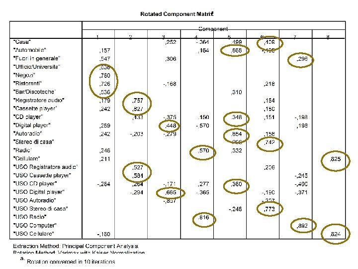
Factor Analysis Number of factors: 8 Second hypothesis: Extraction: Principal Component Analysis Max number of interaction: 25 Rotation : Varimax

Factor Analysis Ratio between component number ADEQUATE and variable number For a set of 17 variables, the ideal number of components is 4 -5. In this case for a set of 24 variables, we have considered 8 components % global explained variance OK About 63% - the optimal range is 60% - 70% Communalities ACCEPTABLE The values vary among 0, 431 and 0, 870

Factor Analysis Scree plot ADEQUATE From the 9 th component , there is little increase in significance explained. “Quite linear slope”

Factor Analysis Interpretation 1. Problems with the 9 th component it’s over. 2. We choosed Varimax option to minimize the number of variables that have elevated saturations for each factor WE CHOOSE THE SECOND HYPOTHESIS

Factor Analysis Interpretation Office/University Shops Restaurants Bars/Discoteque Record player Use record player Cassette player Use cassette player Digital player Use digital player Radio Use radio Car stereo CD player Use CD player Home House stereo Use house stereo OUTSIDE LISTENING STEREO DIGITAL PLAYER RADIO CAR LISTENING HOUSE LISTENING Outside in general Use PC PC Mobile phone Use mobile phone MOBILE PHONE