Methods for flow analysis in ALICE FLOW package

Methods for flow analysis in ALICE FLOW package Ante Bilandzic Trento, 15. 09. 2009

Outline l Anisotropic flow l l Multiparticle azimuthal correlations Methods for flow analysis implemented in ALICE flow package l l l From theorists’ point of view From experimentalists’ point of view 2 -particle methods Multiparticle methods (4 -, 6 - and 8 - particle methods) Genuine multiparticle methods Recent development for ALICE: Q-cumulants Method comparison l l l Idealistic simulations ‘on the fly’ Realistic pp simulations (Pythia) Realistic heavy-ion simulations (Therminator) 2

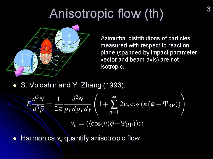
Anisotropic flow (th) Azimuthal distributions of particles measured with respect to reaction plane (spanned by impact parameter vector and beam axis) are not isotropic. l S. Voloshin and Y. Zhang (1996): l Harmonics vn quantify anisotropic flow 3

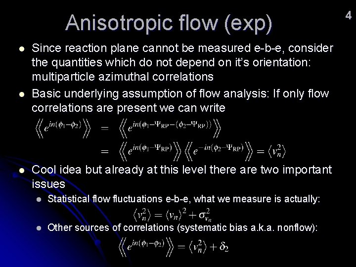
Anisotropic flow (exp) l l l Since reaction plane cannot be measured e-b-e, consider the quantities which do not depend on it’s orientation: multiparticle azimuthal correlations Basic underlying assumption of flow analysis: If only flow correlations are present we can write Cool idea but already at this level there are two important issues l Statistical flow fluctuations e-b-e, what we measure is actually: l Other sources of correlations (systematic bias a. k. a. nonflow): 4

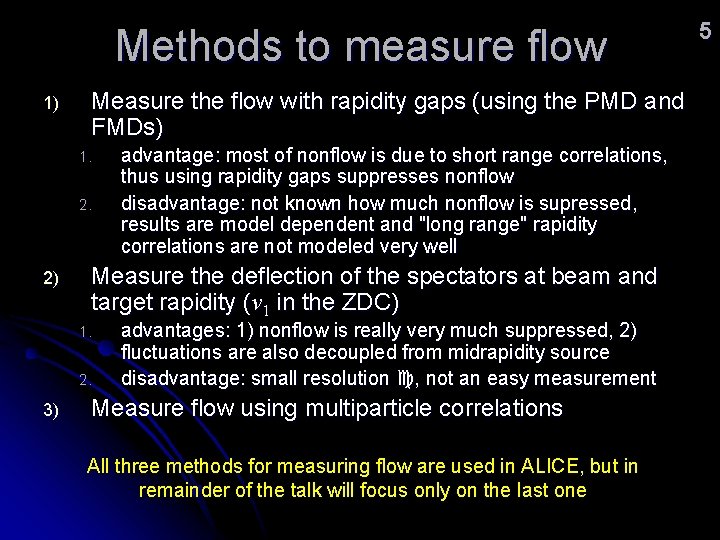
Methods to measure flow 1) Measure the flow with rapidity gaps (using the PMD and FMDs) 1. 2. 2) Measure the deflection of the spectators at beam and target rapidity (v 1 in the ZDC) 1. 2. 3) advantage: most of nonflow is due to short range correlations, thus using rapidity gaps suppresses nonflow disadvantage: not known how much nonflow is supressed, results are model dependent and "long range" rapidity correlations are not modeled very well advantages: 1) nonflow is really very much suppressed, 2) fluctuations are also decoupled from midrapidity source disadvantage: small resolution c, not an easy measurement Measure flow using multiparticle correlations All three methods for measuring flow are used in ALICE, but in remainder of the talk will focus only on the last one 5

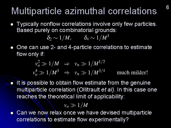
Multiparticle azimuthal correlations l Typically nonflow correlations involve only few particles. Based purely on combinatorial grounds: l One can use 2 - and 4 -particle correlations to estimate flow only if: l It is possible to obtain flow estimate from the genuine multiparticle correlation (Ollitrault et al). In this case one reaches theoretical limit of applicability: l Can we now relax once we have devised multiparticle correlations to estimate flow experimentally? 6

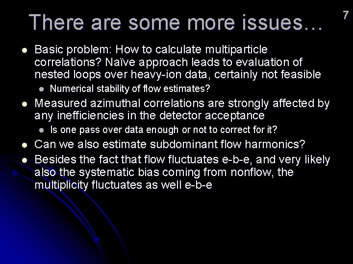
There are some more issues… l Basic problem: How to calculate multiparticle correlations? Naïve approach leads to evaluation of nested loops over heavy-ion data, certainly not feasible l l Measured azimuthal correlations are strongly affected by any inefficiencies in the detector acceptance l l l Numerical stability of flow estimates? Is one pass over data enough or not to correct for it? Can we also estimate subdominant flow harmonics? Besides the fact that flow fluctuates e-b-e, and very likely also the systematic bias coming from nonflow, the multiplicity fluctuates as well e-b-e 7

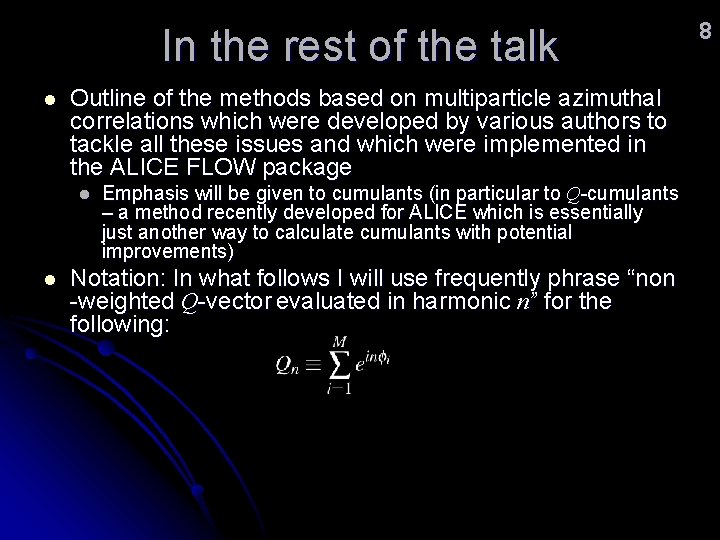
In the rest of the talk l Outline of the methods based on multiparticle azimuthal correlations which were developed by various authors to tackle all these issues and which were implemented in the ALICE FLOW package l l Emphasis will be given to cumulants (in particular to Q-cumulants – a method recently developed for ALICE which is essentially just another way to calculate cumulants with potential improvements) Notation: In what follows I will use frequently phrase “non -weighted Q-vector evaluated in harmonic n” for the following: 8

Methods implemented for ALICE (naming conventions) l l l l MCEP = Monte Carlo Event Plane SP = Scalar Product GFC = Generating Function Cumulants QC = Q-cumulants FQD = Fitting q-distribution LYZ = Lee-Yang Zero (sum and product) LYZEP = Lee-Yang Zero Event Plane Raimond Snellings, Naomi van der Kolk, ab 9

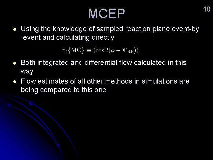
MCEP l Using the knowledge of sampled reaction plane event-by -event and calculating directly l Both integrated and differential flow calculated in this way Flow estimates of all other methods in simulations are being compared to this one l 10

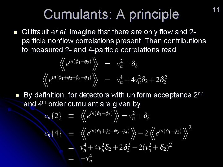
Cumulants: A principle l l Ollitrault et al: Imagine that there are only flow and 2 particle nonflow correlations present. Than contributions to measured 2 - and 4 -particle correlations read By definition, for detectors with uniform acceptance 2 nd and 4 th order cumulant are given by 11

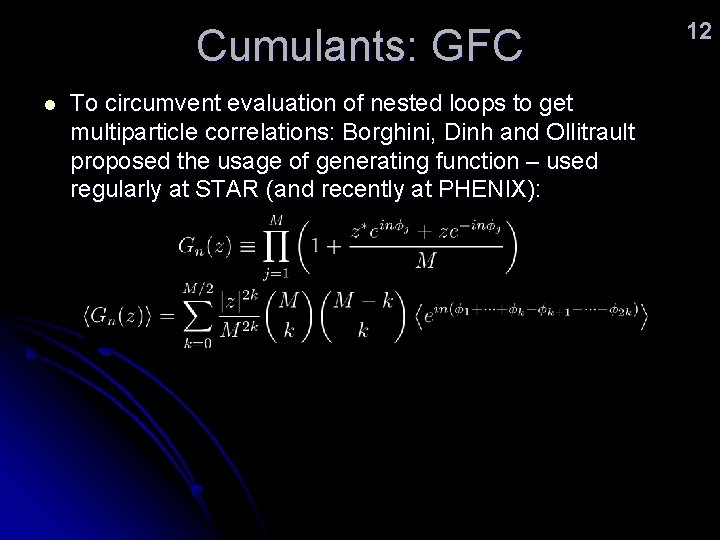
Cumulants: GFC l To circumvent evaluation of nested loops to get multiparticle correlations: Borghini, Dinh and Ollitrault proposed the usage of generating function – used regularly at STAR (and recently at PHENIX): 12

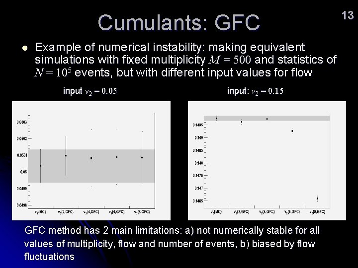
Cumulants: GFC l Example of numerical instability: making equivalent simulations with fixed multiplicity M = 500 and statistics of N = 105 events, but with different input values for flow input v 2 = 0. 05 input: v 2 = 0. 15 GFC method has 2 main limitations: a) not numerically stable for all values of multiplicity, flow and number of events, b) biased by flow fluctuations 13

Cumulants: QC l l l Another approach to circumvent evaluation of nested loops to get multiparticle correlations: Sergei Voloshin’s idea to express multiparticle correlations in terms of expressions involving Q-vectors evaluated (in general) in different harmonics Once you have expressed multiparticle correlations in this way, it is trivial to build up cumulants from them Publication S. Voloshin, R. Snellings, ab “Flow analysis with Q-cumulants” is in preparation 14

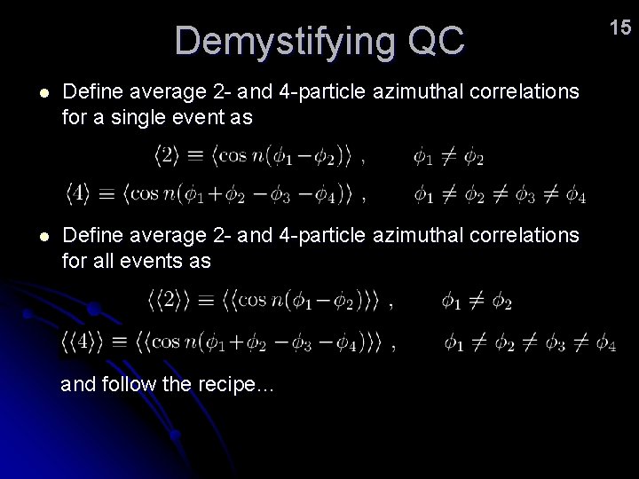
Demystifying QC l Define average 2 - and 4 -particle azimuthal correlations for a single event as l Define average 2 - and 4 -particle azimuthal correlations for all events as and follow the recipe… 15

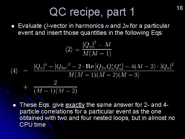
QC recipe, part 1 l l Evaluate Q-vector in harmonics n and 2 n for a particular event and insert those quantities in the following Eqs: These Eqs. give exactly the same answer for 2 - and 4 particle correlations for a particular event as the one obtained with two and four nested loops, but in almost no CPU time 16

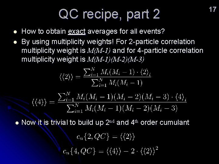
QC recipe, part 2 l l l How to obtain exact averages for all events? By using multiplicity weights! For 2 -particle correlation multiplicity weight is M(M-1) and for 4 -particle correlation multiplicity weight is M(M-1)(M-2)(M-3) Now it is trivial to build up 2 nd and 4 th order cumulant 17

18 Method comparisons (series of plots)

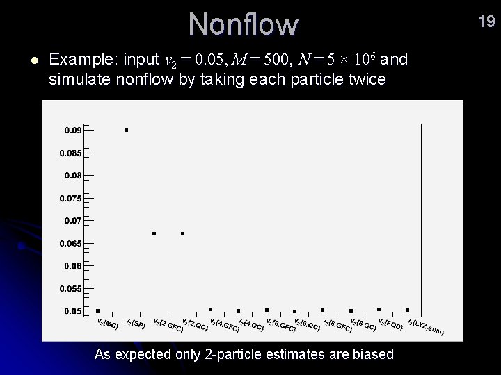
Nonflow l Example: input v 2 = 0. 05, M = 500, N = 5 × 106 and simulate nonflow by taking each particle twice As expected only 2 -particle estimates are biased 19

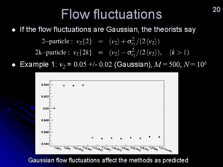
Flow fluctuations l If the flow fluctuations are Gaussian, theorists say l Example 1: v 2 = 0. 05 +/- 0. 02 (Gaussian), M = 500, N = 106 Gaussian flow fluctuations affect the methods as predicted 20

Flow fluctuations l Example 2: v 2 in [0. 04, 0. 06] (uniform), M = 500, N = 9 × 106 Uniform flow fluctuations affect the methods differently as the Gaussian fluctuations 21

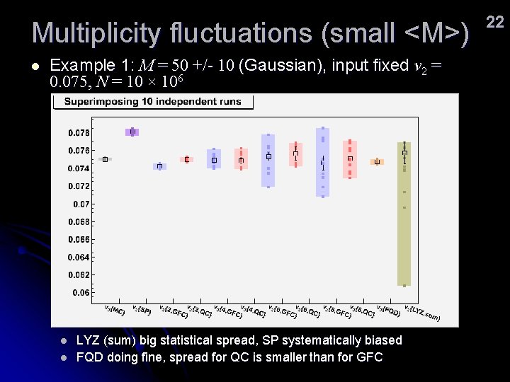
Multiplicity fluctuations (small <M>) l Example 1: M = 50 +/- 10 (Gaussian), input fixed v 2 = 0. 075, N = 10 × 106 l l LYZ (sum) big statistical spread, SP systematically biased FQD doing fine, spread for QC is smaller than for GFC 22

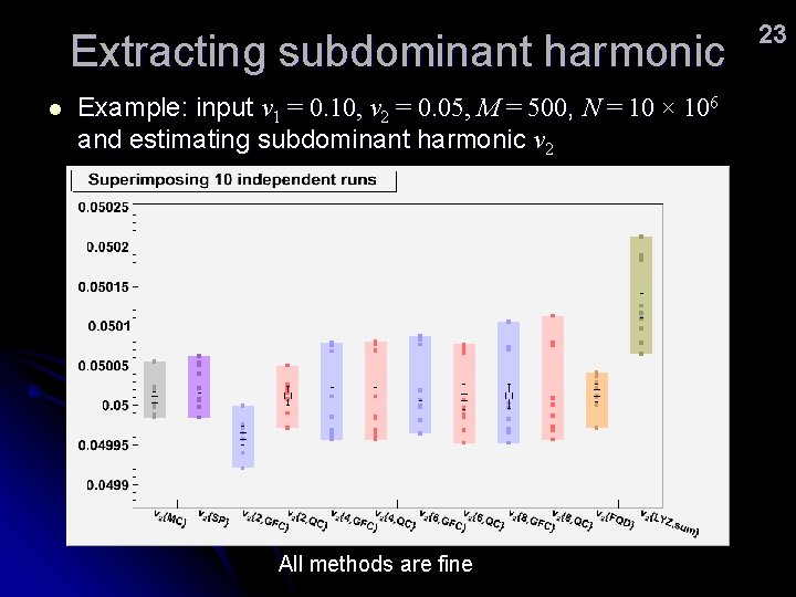
Extracting subdominant harmonic l Example: input v 1 = 0. 10, v 2 = 0. 05, M = 500, N = 10 × 106 and estimating subdominant harmonic v 2 All methods are fine 23

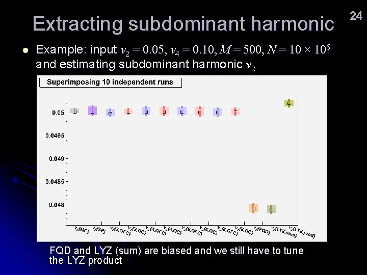
Extracting subdominant harmonic l Example: input v 2 = 0. 05, v 4 = 0. 10, M = 500, N = 10 × 106 and estimating subdominant harmonic v 2 FQD and LYZ (sum) are biased and we still have to tune the LYZ product 24

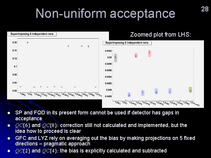
Non-uniform acceptance l To correct for the bias on flow estimates coming from the non-uniform acceptance of the detector, several techniques were proposed by various authors: flattening, recentering, etc. l l l Ollitrault et al proposed evaluating generating functions along fixed directions in the laboratory frame and averaging the results obtained for those directions: l l l require additional run over data some of them not applicable for detectors with gaps in azimuthal acceptance (e. g. flattening) works fine for GFC and LYZ no need for an additional run over data Recent: For Q-cumulants it is possible explicitly to calculate and subtract the bias coming from the nonuniform acceptance l l applicable to all types of non-uniform acceptance one run over data enough 25

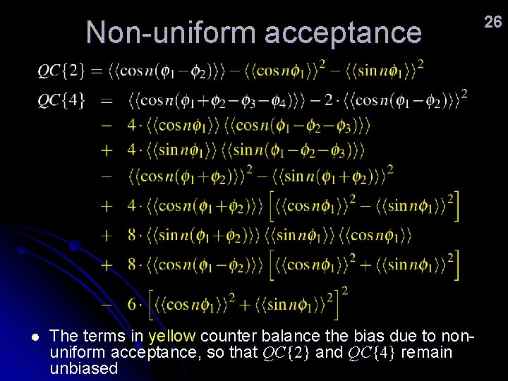
Non-uniform acceptance l The terms in yellow counter balance the bias due to nonuniform acceptance, so that QC{2} and QC{4} remain unbiased 26

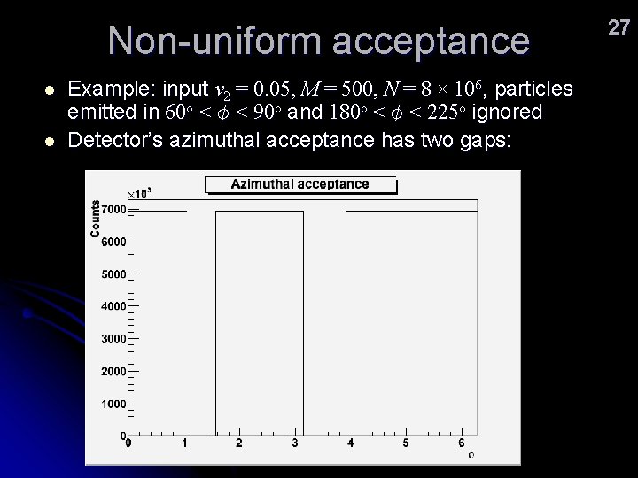
Non-uniform acceptance l l Example: input v 2 = 0. 05, M = 500, N = 8 × 106, particles emitted in 60 o < f < 90 o and 180 o < f < 225 o ignored Detector’s azimuthal acceptance has two gaps: 27

Non-uniform acceptance Zoomed plot from LHS: l l SP and FQD in its present form cannot be used if detector has gaps in acceptance QC{6} and QC{8}: correction still not calculated and implemented, but the idea how to proceed is clear GFC and LYZ rely on averaging out the bias by making projections on 5 fixed directions – pragmatic approach QC{2} and QC{4}: the bias is explicitly calculated and subtracted 28

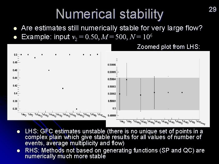
Numerical stability l l Are estimates still numerically stable for very large flow? Example: input v 2 = 0. 50, M = 500, N = 106 Zoomed plot from LHS: l l LHS: GFC estimates unstable (there is no unique set of points in a complex plain which give stable results for all values of number of events, average multiplicity and flow) RHS: Methods not based on generating functions (SP and QC) are numerically much more stable 29

QC factbook l l l l Possible to get both integrated and differential flow in a single run Not biased by interference between different harmonics: can be applied to extract subdominant harmonics Not biased by interference between different order estimates for the same harmonic (e. g. you do not need the knowledge of the 8 th order estimate to calculate the 2 nd order estimate) Not biased by multiplicity fluctuations: compared to GFC improved results for peripheral collisions Not biased by numerical errors: compared to GFC no need to tune interpolating parameters (e. g. r 0 for GFC, QC has no parameters) Detector effects can be quantified and corrected for in a single run over data even for the detectors with gaps in azimuthal acceptance Biased by flow fluctuations 30

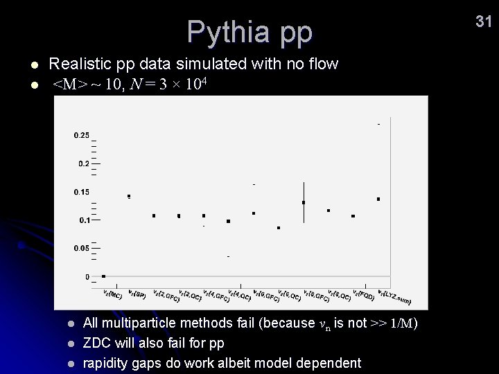
Pythia pp l l Realistic pp data simulated with no flow <M> ~ 10, N = 3 × 104 l l l All multiparticle methods fail (because vn is not >> 1/M) ZDC will also fail for pp rapidity gaps do work albeit model dependent 31

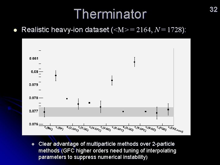
Therminator l Realistic heavy-ion dataset (<M> = 2164, N = 1728): l Clear advantage of multiparticle methods over 2 -particle methods (GFC higher orders need tuning of interpolating parameters to suppress numerical instability) 32

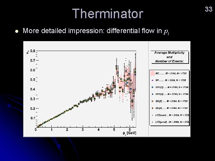
Therminator l More detailed impression: differential flow in pt 33

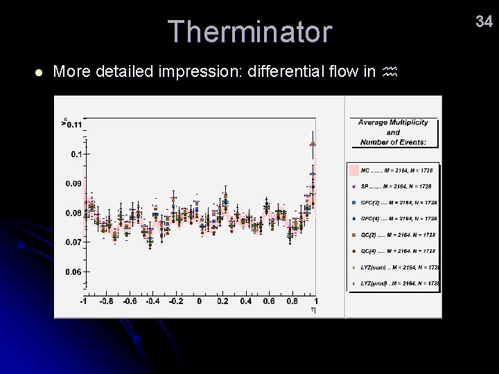
Therminator l More detailed impression: differential flow in h 34

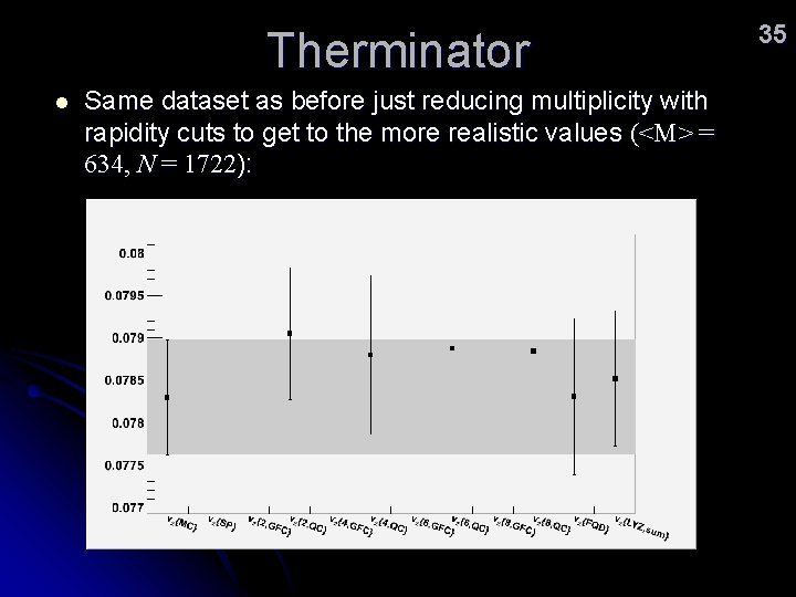
Therminator l Same dataset as before just reducing multiplicity with rapidity cuts to get to the more realistic values (<M> = 634, N = 1722): 35

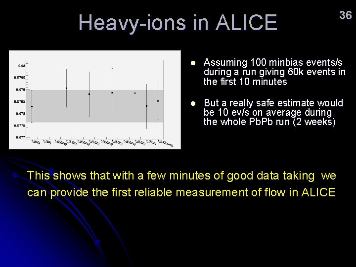
Heavy-ions in ALICE 36 l Assuming 100 minbias events/s during a run giving 60 k events in the first 10 minutes l But a really safe estimate would be 10 ev/s on average during the whole Pb. Pb run (2 weeks) This shows that with a few minutes of good data taking we can provide the first reliable measurement of flow in ALICE

37 Thanks!

38 Backup slides

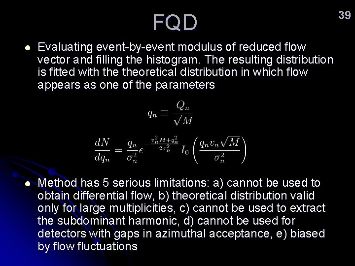
FQD l Evaluating event-by-event modulus of reduced flow vector and filling the histogram. The resulting distribution is fitted with theoretical distribution in which flow appears as one of the parameters l Method has 5 serious limitations: a) cannot be used to obtain differential flow, b) theoretical distribution valid only for large multiplicities, c) cannot be used to extract the subdominant harmonic, d) cannot be used for detectors with gaps in azimuthal acceptance, e) biased by flow fluctuations 39

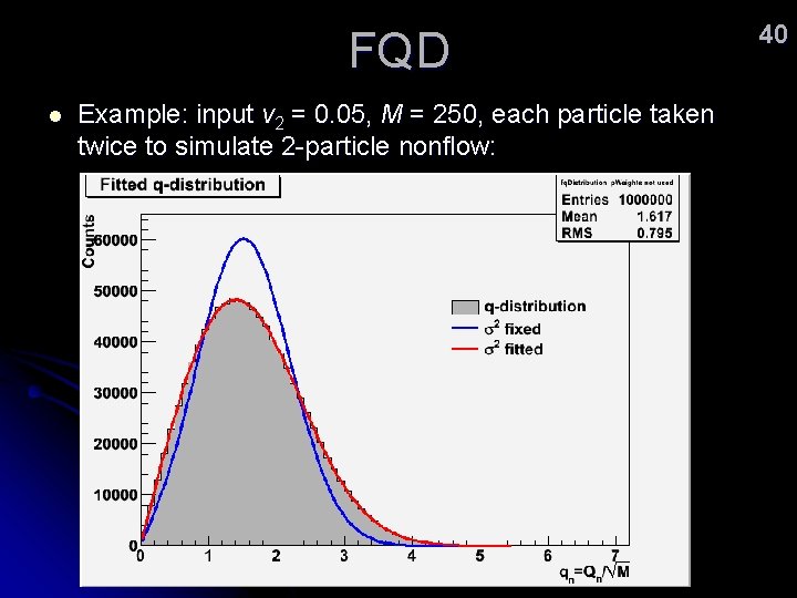
FQD l Example: input v 2 = 0. 05, M = 250, each particle taken twice to simulate 2 -particle nonflow: 40

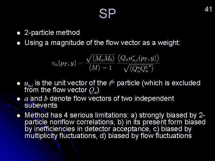
SP l l l 41 2 -particle method Using a magnitude of the flow vector as a weight: un, i is the unit vector of the ith particle (which is excluded from the flow vector Qn) a and b denote flow vectors of two independent subevents Method has 4 serious limitations: a) strongly biased by 2 particle nonflow correlations, b) in its present form biased by inefficiencies in detector acceptance, c) biased by multiplicity fluctuations, d) biased by flow fluctuations

LYZ and LYZEP l l l Introduced by Ollitrault et al Gives genuine multiparticle estimate, both for integrated and differential flow Two version implemented – sum and product LYZEP additionally provides the event plane and it is based on LYZ (sum) The method has 3 main limitations: a) one pass over data is not enough, b) not numerically stable for all flow values, c) biased by flow fluctuations 42

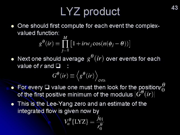
LYZ product l One should first compute for each event the complexvalued function: l Next one should average value of r and q : l For every q value one must then look for the position of the first positive minimum of the modulus l This is the Lee-Yang zero and an estimate of the integrated flow is given now by over events for each 43

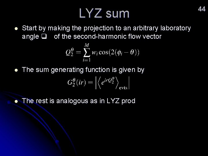
LYZ sum l Start by making the projection to an arbitrary laboratory angle q of the second-harmonic flow vector l The sum generating function is given by l The rest is analogous as in LYZ prod 44

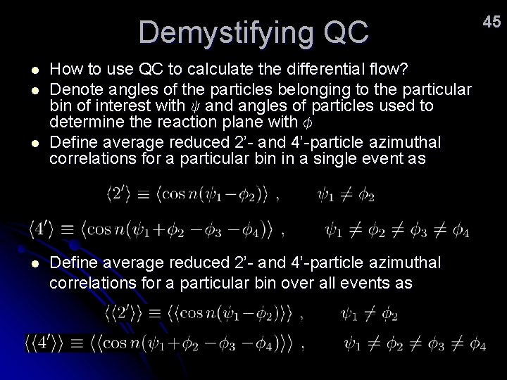
Demystifying QC l l How to use QC to calculate the differential flow? Denote angles of the particles belonging to the particular bin of interest with y and angles of particles used to determine the reaction plane with f Define average reduced 2’- and 4’-particle azimuthal correlations for a particular bin in a single event as Define average reduced 2’- and 4’-particle azimuthal correlations for a particular bin over all events as 45

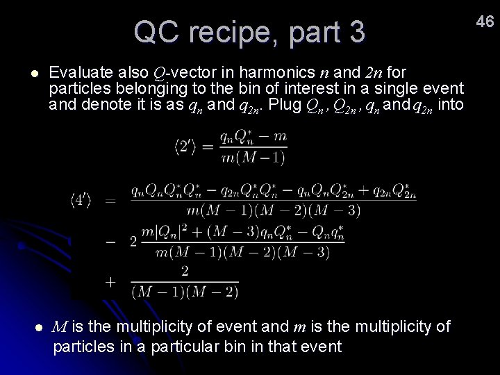
QC recipe, part 3 l l Evaluate also Q-vector in harmonics n and 2 n for particles belonging to the bin of interest in a single event and denote it is as qn and q 2 n. Plug Qn , Q 2 n , qn and q 2 n into M is the multiplicity of event and m is the multiplicity of particles in a particular bin in that event 46

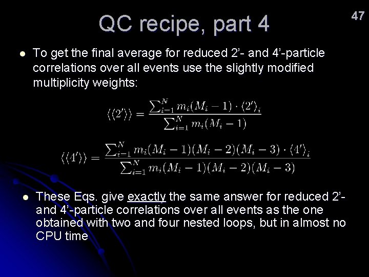
QC recipe, part 4 l l To get the final average for reduced 2’- and 4’-particle correlations over all events use the slightly modified multiplicity weights: These Eqs. give exactly the same answer for reduced 2’and 4’-particle correlations over all events as the one obtained with two and four nested loops, but in almost no CPU time 47

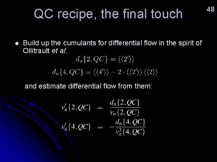
QC recipe, the final touch l Build up the cumulants for differential flow in the spirit of Ollitrault et al: and estimate differential flow from them: 48