Methods for Dummies 2009 Dynamic Causal Modelling Part

Methods for Dummies 2009 Dynamic Causal Modelling Part I: Theory 18 th February 2009 Stephanie Burnett Christian Lambert

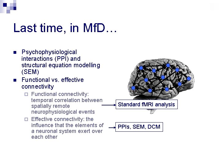
Last time, in Mf. D… n n Psychophysiological interactions (PPI) and structural equation modelling (SEM) Functional vs. effective connectivity Functional connectivity: temporal correlation between spatially remote neurophysiological events ¨ Effective connectivity: the influence that the elements of a neuronal system exert over each other ¨ Standard f. MRI analysis PPIs, SEM, DCM

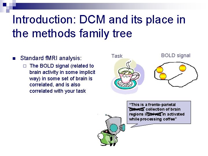
Introduction: DCM and its place in the methods family tree n Standard f. MRI analysis: ¨ Task BOLD signal The BOLD signal (related to brain activity in some implicit way) in some set of brain is correlated, and is also correlated with your task “This is a fronto-parietal network collection of brain regions involved in activated while processing coffee”

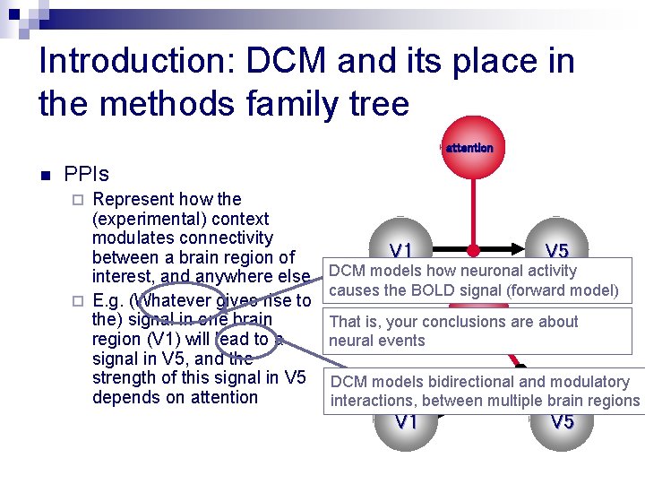
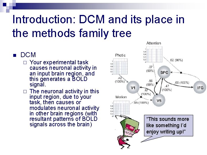
Introduction: DCM and its place in the methods family tree attention n PPIs Represent how the (experimental) context modulates connectivity between a brain region of interest, and anywhere else ¨ E. g. (Whatever gives rise to the) signal in one brain region (V 1) will lead to a signal in V 5, and the strength of this signal in V 5 depends on attention ¨ V 1 V 5 DCM models how neuronal activity causes the BOLD signal (forward model) attention are about That is, your conclusions neural events DCM models bidirectional and modulatory interactions, between multiple brain regions V 1 V 5

Introduction: DCM and its place in the methods family tree n DCM Your experimental task causes neuronal activity in an input brain region, and this generates a BOLD signal. ¨ The neuronal activity in this input region, due to your task, then causes or modulates neuronal activity in other brain regions (with resultant patterns of BOLD signals across the brain) ¨ “This sounds more like something I’d enjoy writing up!”

DCM basics n DCM models interactions between neuronal populations ¨ n f. MRI, MEG, EEG The aim is to estimate, and make inferences about: 1. 2. The coupling among brain areas How that coupling is influenced by changes in experimental context

DCM basics n n n DCM starts with a realistic model of how brain regions interact and where the inputs can come in Adds a forward model of how neuronal activity causes the signals you observe (e. g. BOLD) …and estimates the parameters in your model (effective connectivity), given your observed data Neural and hemodynamic models (more on this in a few minutes)

DCM basics n n n Inputs State variables Outputs

DCM basics n Inputs In functional connectivity models (e. g. standard f. MRI analysis), conceptually your input could have entered anywhere ¨ In effective connectivity models (e. g. DCM), input only enters at certain places ¨

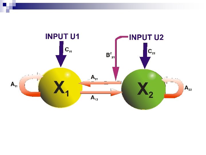
DCM basics n Inputs can exert their influence in two ways: 1. Direct influence n e. g. visual input to V 1 ¨ 2. Vicarious (indirect) influence n e. g. attentional modulation of the coupling between V 1 and V 5 ¨

DCM basics n State variables ¨ Neuronal activities, and other neuro- or bio -physical variables needed to form the outputs n n Neuronal priors Haemodynamic priors What you’re modelling is how the inputs modulate the coupling among these state variables

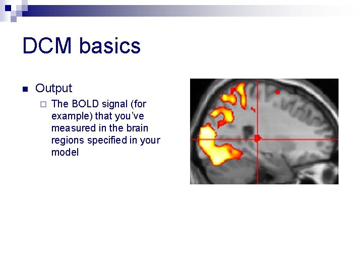
DCM basics n Output ¨ The BOLD signal (for example) that you’ve measured in the brain regions specified in your model

Dynamic Modelling (i) n Generate equations to model the dynamics of physical systems. n These will be LINEAR or NON-LINEAR n Linear models provide good approximation n However neuronal dynamics are non-linear in nature

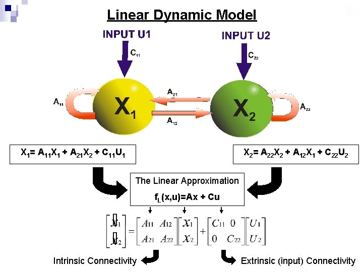
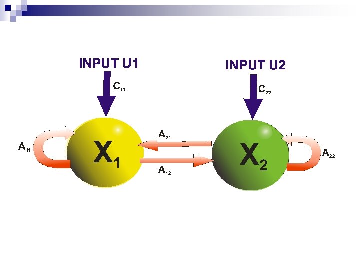
Linear Dynamic Model X 1= A 11 X 1 + A 21 X 2 + C 11 U 1 X 2= A 22 X 2 + A 12 X 1 + C 22 U 2 The Linear Approximation f. L(x, u)=Ax + Cu Intrinsic Connectivity Extrinsic (input) Connectivity

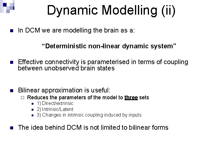
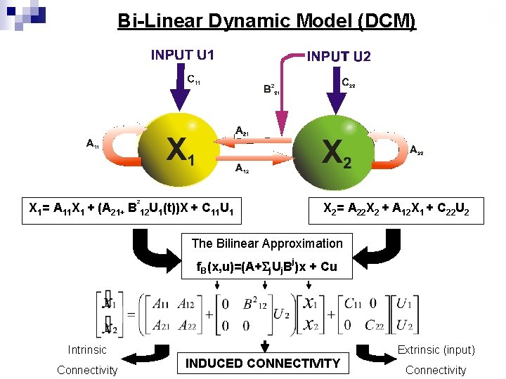
Dynamic Modelling (ii) n In DCM we are modelling the brain as a: “Deterministic non-linear dynamic system” n Effective connectivity is parameterised in terms of coupling between unobserved brain states n Bilinear approximation is useful: ¨ Reduces the parameters of the model to three sets n n 1) Direct/extrinsic 2) Intrinsic/Latent 3) Changes in intrinsic coupling induced by inputs The idea behind DCM is not limited to bilinear forms

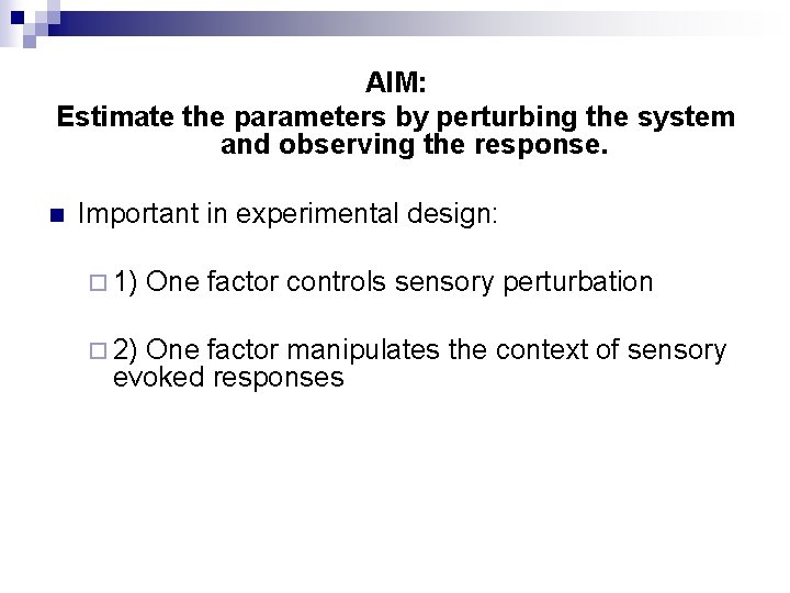
AIM: Estimate the parameters by perturbing the system and observing the response. n Important in experimental design: ¨ 1) ¨ 2) One factor controls sensory perturbation One factor manipulates the context of sensory evoked responses

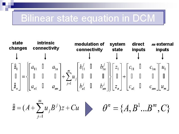
Bi-Linear Dynamic Model (DCM) 2 X 1= A 11 X 1 + (A 21+ B 12 U 1(t))X + C 11 U 1 X 2= A 22 X 2 + A 12 X 1 + C 22 U 2 The Bilinear Approximation j f. B(x, u)=(A+ j. Uj. B )x + Cu Intrinsic Connectivity Extrinsic (input) INDUCED CONNECTIVITY Connectivity

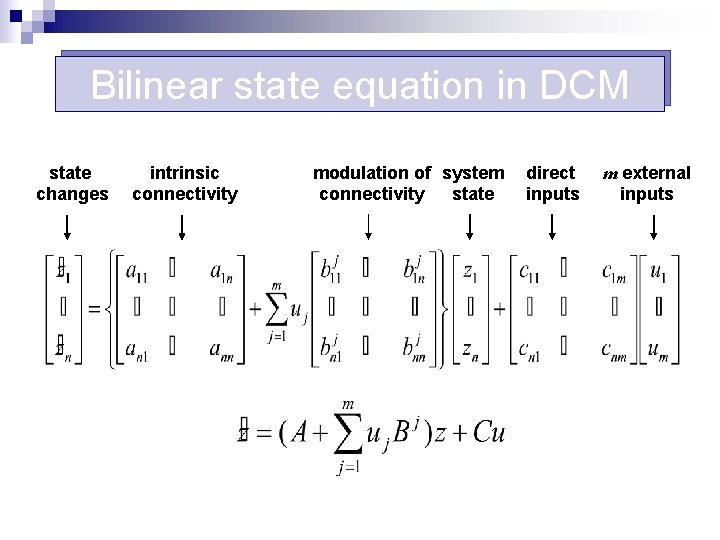
Bilinear state equation in DCM state changes intrinsic connectivity modulation of system connectivity state direct inputs m external inputs

Bilinear state equation in DCM state changes intrinsic connectivity modulation of connectivity system state direct inputs m external inputs

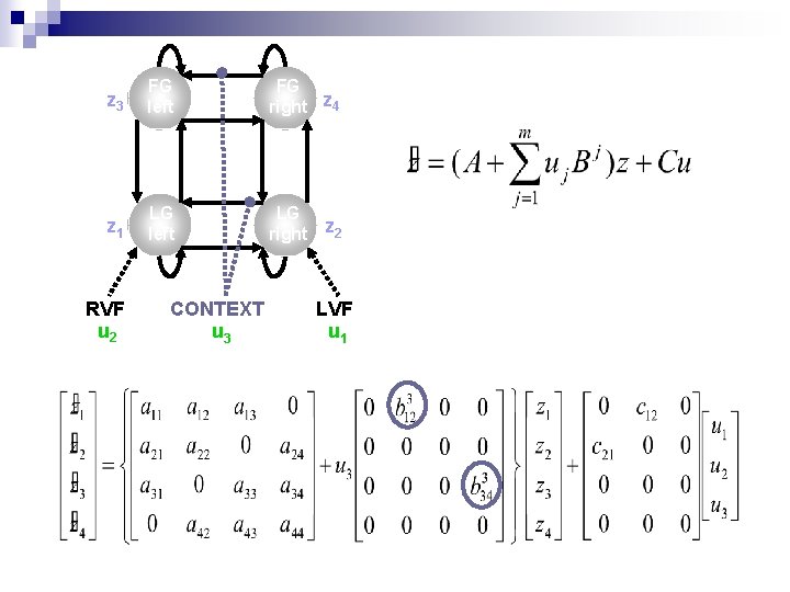
z 3 FG left FG right z 4 z 1 LG left LG right z 2 RVF u 2 CONTEXT u 3 LVF u 1

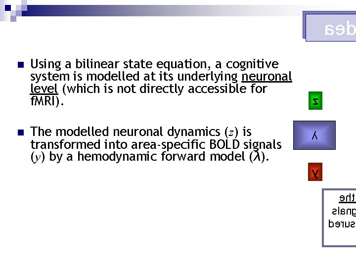
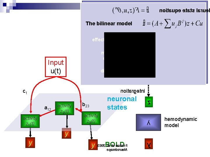
ae n n Using a bilinear state equation, a cognitive system is modelled at its underlying neuronal level (which is not directly accessible for f. MRI). The modelled neuronal dynamics (z) is transformed into area-specific BOLD signals (y) by a hemodynamic forward model (λ). z λ y eht slan derus

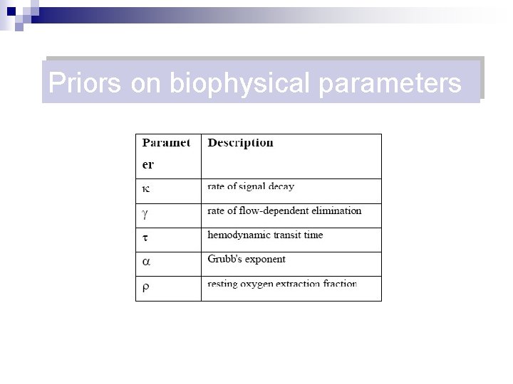
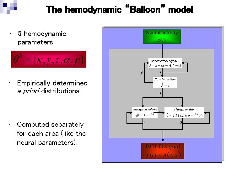
Priors on biophysical parameters

The hemodynamic “Balloon” model • 5 hemodynamic parameters: Vasodilatory signal • Empirically determined a priori distributions. • Computed separately for each area (like the neural parameters).

noitauqe etats larue The bilinear model effective connectivity modulation of connectivity Input u(t) direct inputs c 1 noitargetni a 12 activity z 2(t) activity z 1(t) neuronal states b 23 activity z 3(t) z λ y y . la te notsir. F y , 3002 BOLD egam. Iorue. N y hemodynamic model

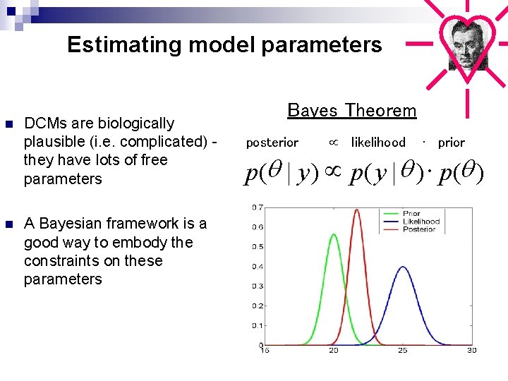
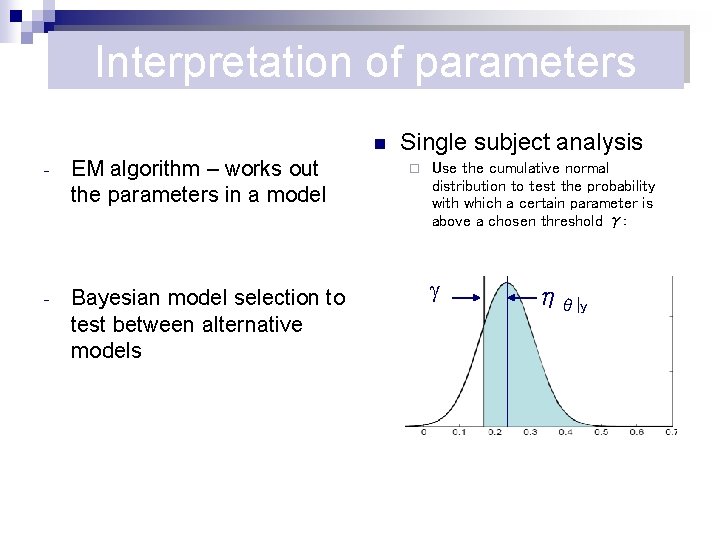
Estimating model parameters n n DCMs are biologically plausible (i. e. complicated) they have lots of free parameters A Bayesian framework is a good way to embody the constraints on these parameters Bayes Theorem posterior likelihood ∙ prior p(q | y ) p( y | q ) × p(q )

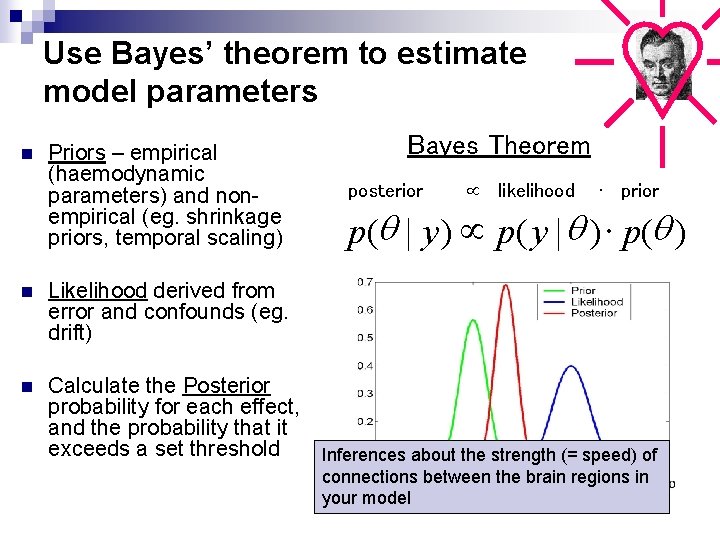
Use Bayes’ theorem to estimate model parameters n Priors – empirical (haemodynamic parameters) and nonempirical (eg. shrinkage priors, temporal scaling) Bayes Theorem posterior likelihood ∙ prior p(q | y ) p( y | q ) × p(q ) n Likelihood derived from error and confounds (eg. drift) n Calculate the Posterior probability for each effect, and the probability that it exceeds a set threshold Inferences about the strength (= speed) of connections between the brain regions in your model

Interpretation of parameters n - EM algorithm – works out the parameters in a model - Bayesian model selection to test between alternative models Single subject analysis ¨ Use the cumulative normal distribution to test the probability with which a certain parameter is above a chosen threshold γ: ηθ|y

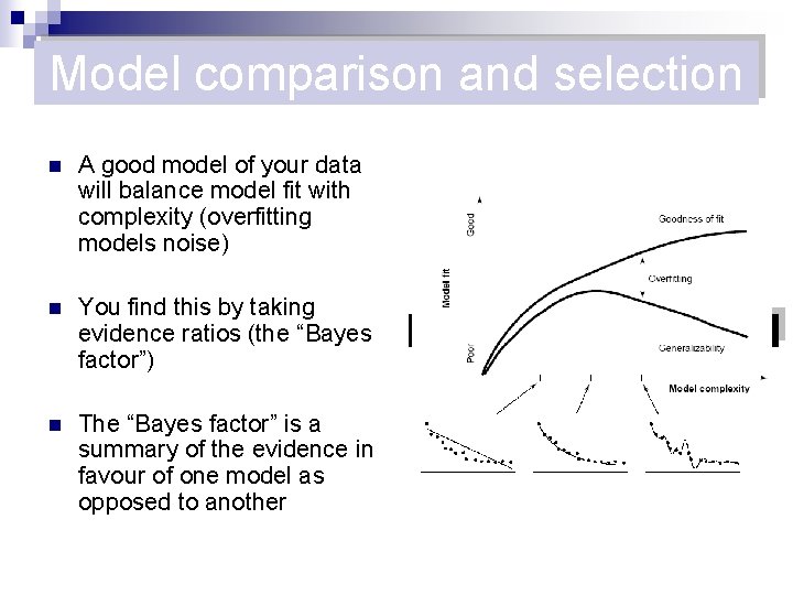
Model comparison and selection n A good model of your data will balance model fit with complexity (overfitting models noise) n You find this by taking evidence ratios (the “Bayes factor”) n The “Bayes factor” is a summary of the evidence in favour of one model as opposed to another

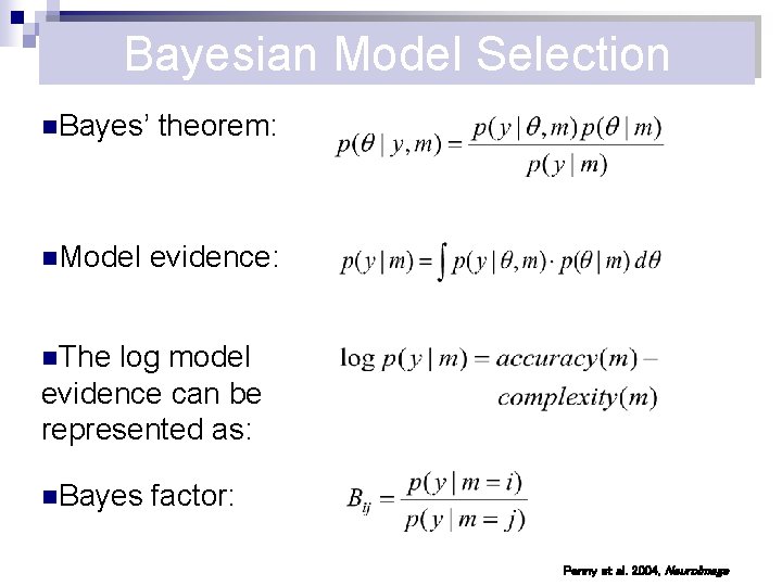
Bayesian Model Selection n. Bayes’ n. Model theorem: evidence: n. The log model evidence can be represented as: n. Bayes factor: Penny et al. 2004, Neuro. Image

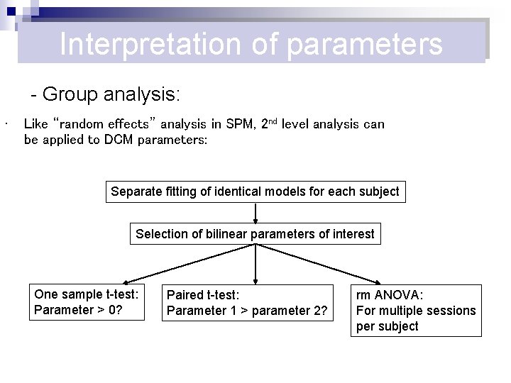
Interpretation of parameters - Group analysis: • Like “random effects” analysis in SPM, 2 nd level analysis can be applied to DCM parameters: Separate fitting of identical models for each subject Selection of bilinear parameters of interest One sample t-test: Parameter > 0? Paired t-test: Parameter 1 > parameter 2? rm ANOVA: For multiple sessions per subject

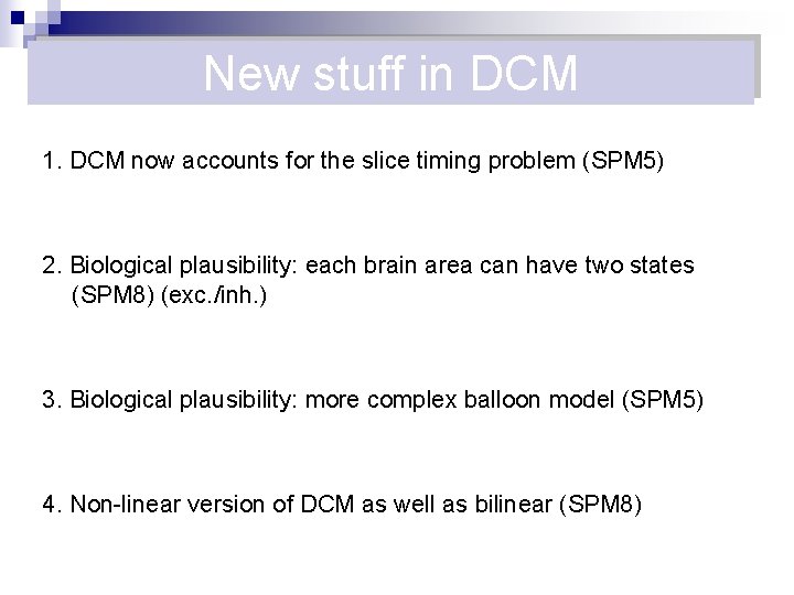
New stuff in DCM n 1. DCM now accounts for the slice timing problem

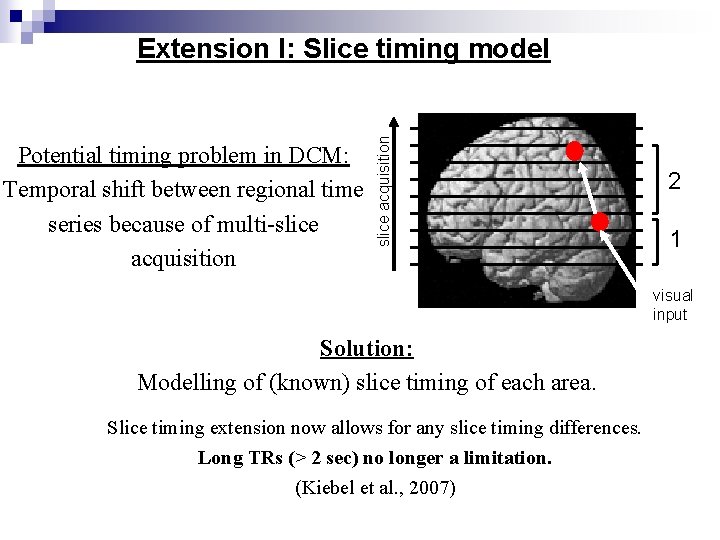
Potential timing problem in DCM: Temporal shift between regional time series because of multi-slice acquisition Extension I: Slice timing model 2 1 visual input Solution: Modelling of (known) slice timing of each area. Slice timing extension now allows for any slice timing differences. Long TRs (> 2 sec) no longer a limitation. (Kiebel et al. , 2007)

New stuff in DCM 1. DCM now accounts for the slice timing problem (SPM 5) 2. Biological plausibility: each brain area can have two states (SPM 8) (exc. /inh. )

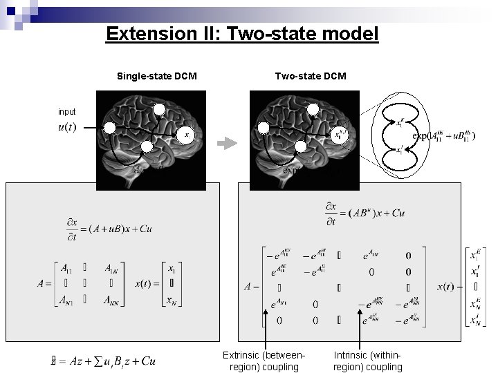
Extension II: Two-state model Single-state DCM Two-state DCM input Extrinsic (betweenregion) coupling Intrinsic (withinregion) coupling

New stuff in DCM 1. DCM now accounts for the slice timing problem (SPM 5) 2. Biological plausibility: each brain area can have two states (SPM 8) (exc. /inh. ) 3. Biological plausibility: more complex balloon model (SPM 5) 4. Non-linear version of DCM as well as bilinear (SPM 8)

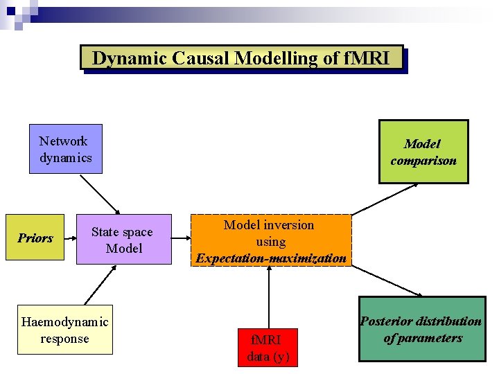
Dynamic Causal Modelling of f. MRI Network dynamics Priors State space Model Haemodynamic response Model comparison Model inversion using Expectation-maximization f. MRI data (y) Posterior distribution of parameters

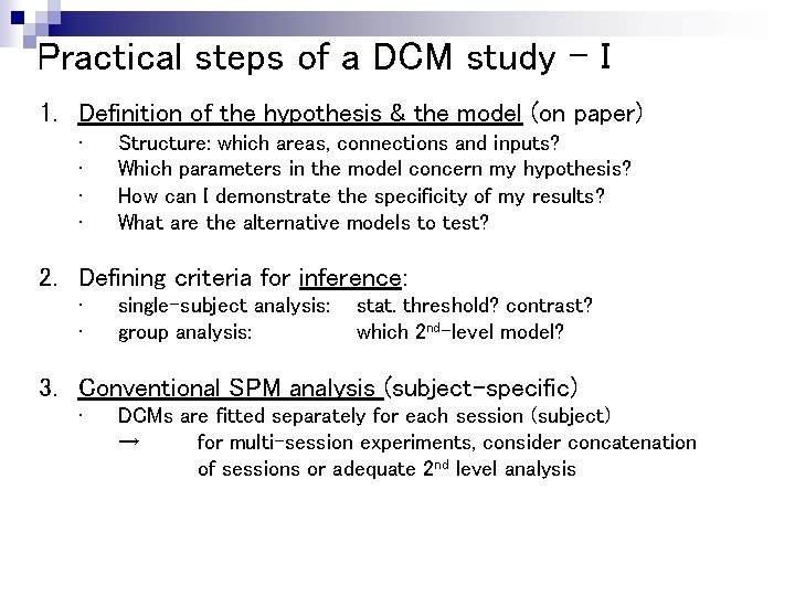
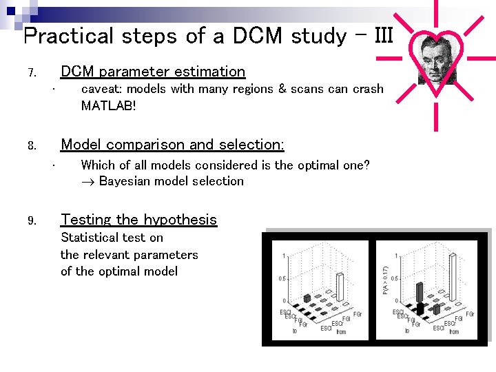
Practical steps of a DCM study - I 1. Definition of the hypothesis & the model (on paper) • • Structure: which areas, connections and inputs? Which parameters in the model concern my hypothesis? How can I demonstrate the specificity of my results? What are the alternative models to test? 2. Defining criteria for inference: • • single-subject analysis: group analysis: stat. threshold? contrast? which 2 nd-level model? 3. Conventional SPM analysis (subject-specific) • DCMs are fitted separately for each session (subject) → for multi-session experiments, consider concatenation of sessions or adequate 2 nd level analysis

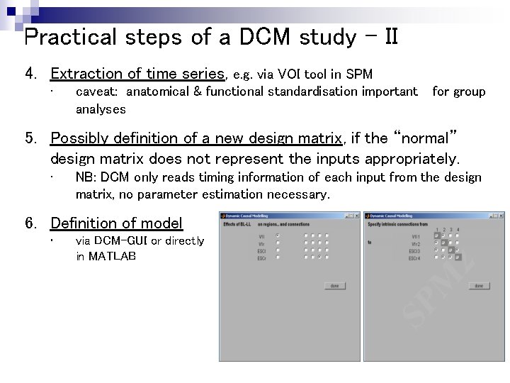
Practical steps of a DCM study - II 4. Extraction of time series, e. g. via VOI tool in SPM • caveat: anatomical & functional standardisation important analyses for group 5. Possibly definition of a new design matrix, if the “normal” design matrix does not represent the inputs appropriately. • NB: DCM only reads timing information of each input from the design matrix, no parameter estimation necessary. 6. Definition of model • via DCM-GUI or directly in MATLAB

Practical steps of a DCM study - III DCM parameter estimation 7. • Model comparison and selection: 8. • 9. caveat: models with many regions & scans can crash MATLAB! Which of all models considered is the optimal one? Bayesian model selection Testing the hypothesis Statistical test on the relevant parameters of the optimal model

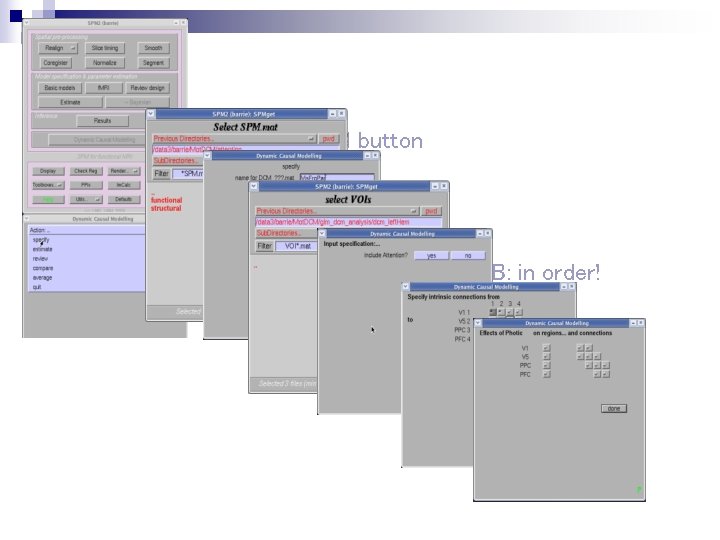
DCM button ‘specify’ NB: in order!

Summary n DCM is NOT EXPLORATORY n Used to test the hypothesis that motivated the experimental design ¨ BUILD A MODEL TO EXPRESS HYPOTHESIS IN TERMS OF NEURAL CONNECTIVITY n The GLM used in typical f. MRI data analysis uses the same architecture as DCM but embodies more assumptions n Note: In DCM a “Strong Connection” means an influence that is expressed quickly or with a small time constant. n When constructing experiments, consider whether you want to use DCM early n When in doubt, ask the experts………

REFERENCES n Karl J. Friston. Dynamic Causal Modelling. Human brain function. Chapter 22. Second Edition. http: //www. fil. ion. ucl. ac. uk/spm/doc/books/hbf 2/ n K. J Friston, L. Harrison and W. Penny. Dynamic Causal Modelling. Neuroimage 2003; 19: 1273 -1302. n SPM Manual n Last year’s presentation

ANY QUESTIONS? ? ?