Methods for Dummies 2 nd level analysis Dummies

Methods for Dummies 2 nd level analysis Dummies: Fraser Aitken & Lara Gregorians Expert: Guillaume Flandin

Structure ● ● 1 st level analysis recap What is 2 nd level analysis? Fixed and random effects How to carry out random effects analysis

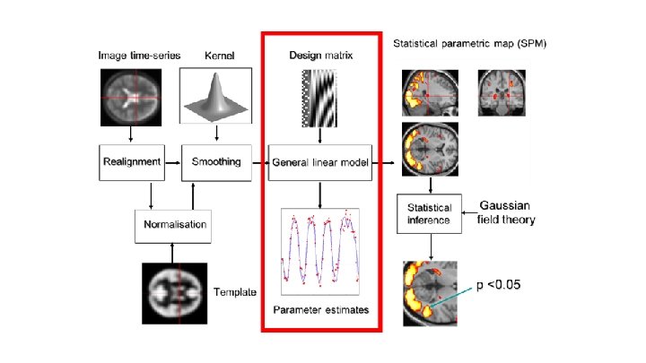
Time-series per voxel, per participant GLM: Y= β 0+β 1 X 1+ ϵ Convolution: Contrasts:

What is 2 nd level analysis? ● 2 nd level analysis = looking at across subject effects as opposed to single subject effect ● Significant differences in activation between different levels of X are unlikely to be manifest identically in all individuals. Therefore, we might ask: ○ Is this contrast in activation different on average between groups? e. g. males vs. females? ○ Is this contrast in activation seen on average in the population?

What is 2 nd level analysis? ● We need to look at which voxels are showing a significant activation difference between levels of X consistently within a group. To do this, we need to consider: ○ The average contrast effect across our sample ○ The variation of this contrast effect ○ T-tests involve mean divided by standard error of mean

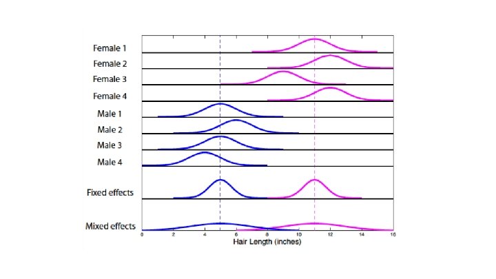
Fixed vs. Random effects Fixed effects model Random effects model Comparing effect size to within subject variability (i. e. not an inference about the pop. ). Comparing group effect to between subject variability (i. e. an inference about the pop. ). Only one source of variation - measurement error (true response magnitude is fixed). Models multiple sources of variation - measurement error AND true response magnitude (i. e. individual difference, which is random). Levels not drawn from random sample; always the same e. g. Drug use Y/N. Levels randomly sampled from population e. g. participant selected at random. CANNOT generalise to unobserved subjects. CAN generalise to unobserved subjects.

Worked example For group of N = 12 subjects x 50 scans = 600 Effect sizes c = [4, 3, 2, 1, 1, 2, 3, 3, 3, 2, 4, 4] Subject 1 Effect size c = 4 for given voxel Within subject variability = 0. 9 Within subject variability = [0. 9, 1. 2, 1. 5, 0. 4, 0. 7, 0. 8, 2. 1, 1. 8, 0. 7, 1. 1] Mean group effect M = 2. 67 Average within subject variability (SD) σw 2 = 1. 04 Standard Error Mean (SEM) = σw 2 /(sqrt(N))=0. 04 t=M/SEM = 62. 7, p=10 -51

Fixed vs. Random effects Fixed effects model Random effects model Comparing effect size to within subject variability (i. e. not an inference about the pop. ). Comparing group effect to between subject variability (i. e. an inference about the pop. ). Only one source of variation - measurement error (true response magnitude is fixed). Models multiple sources of variation - measurement error AND true response magnitude (i. e. individual difference, which is random). Levels not drawn from random sample; always the same e. g. Drug Y/N. Levels randomly sampled from population e. g. participant selected at random. CANNOT generalise to unobserved subjects. CAN generalise to unobserved subjects.

How to carry out random effects analysis? ● Synonymous with ‘mixed effects models’. ● Assumes our sample is a set of individuals taken at random from the population of interest. ● To do this we need to consider the between subject variance AND within subject variance – and estimate the likely variance of the population from which our sample is derived.

Hierarchical models ● Estimate subject and group stats at the same time via iterative looping ● Gold standard in terms of accuracy but…. . . ● Computationally intensive, and not always practical! (e. g. adding in subjects means the entire estimation process has to start from scratch again)

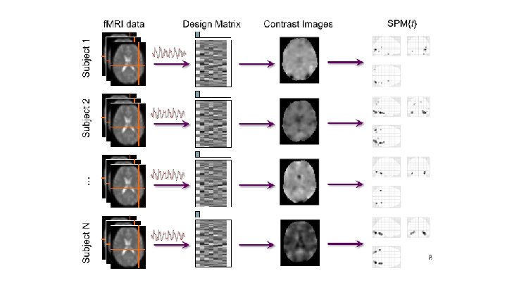
Summary stats

Worked example For group of N = 12 subjects Effect sizes c = [4, 3, 2, 1, 1, 2, 3, 3, 3, 2, 4, 4] Mean group effect m = 2. 67 Between subject variability (SD) σb 2 = 1. 07 Standard Error Mean (SEM) = σb 2 /(sqrt(N))=0. 31 t=M/SEM = 8. 61, p=10 -6 Subject 1 Effect size c = 4 for given voxel

Overview ● 2 nd level analysis = looking at effects across subjects. ● Between-subject variance is much greater than within-subject variance. We need to consider both aspects of variance to make any inferences about the wider population, rather than just our sample. ● As the population variance is much greater than the within-subjects variance, fixed effects analysis ‘overestimates’ the significance of effects – random effects analysis is more conservative, highlighting the greater effects that may be seen across the population. ● Using fixed effects isn’t necessarily wrong, but might not be useful.

Thank you

Helpful resources SPM course videos https: //www. fil. ion. ucl. ac. uk/spm/course/video/#Group Principles of f. MRI [series] https: //www. youtube. com/watch? v=ZLTr 1 KSMKY&list=PLf. XA 4 op. IOVr. GHnc. HRx. I 3 Qa 5 Ge. CSudwmx. M