Mesoscale Probabilistic Prediction over the Northwest An Overview

Mesoscale Probabilistic Prediction over the Northwest: An Overview Cliff Mass University of Washington

Mesoscale Probabilistic Prediction • By the late 1990’s, we had a good idea of the benefits of high resolution. • It was clear that initial condition and physics uncertainty was large. • We were also sitting on an unusual asset due to our work evaluating major NWP centers: realtime initializations and forecasts from NWP centers around the world. • Also, inexpensive UNIX clusters became available.
 Abbreviation/Model/Source Type avn, Global Forecast")
“Native” Models/Analyses Available Resolution (~ @ 45 N ) Abbreviation/Model/Source Type avn, Global Forecast System (GFS), Spectral T 254 / L 64 ~55 km National Centers for Environmental Prediction cmcg, Global Environmental Multi-scale (GEM), Computational Distributed 1. 0 / L 14 ~80 km Objective Analysis SSI 3 D Var Finite Diff 0. 9 /L 28 1. 25 / L 11 ~70 km ~100 km 3 D Var Finite Diff. 32 km / L 45 90 km / L 37 SSI 3 D Var Spectral T 239 / L 29 ~60 km 1. 0 / L 11 ~80 km 3 D Var Spectral T 106 / L 21 ~135 km 1. 25 / L 13 ~100 km OI Spectral T 239 / L 30 Fleet Numerical Meteorological & Oceanographic Cntr. ~60 km 1. 0 / L 14 ~80 km OI tcwb, Global Forecast System, 1. 0 / L 11 ~80 km OI Canadian Meteorological Centre eta, limited-area mesoscale model, National Centers for Environmental Prediction gasp, Global Analysi. S and Prediction model, Australian Bureau of Meteorology jma, Global Spectral Model (GSM), Japan Meteorological Agency ngps, Navy Operational Global Atmos. Pred. System, Taiwan Central Weather Bureau ukmo, Unified Model, United Kingdom Meteorological Office Spectral T 79 / L 18 ~180 km Finite Diff. 5/6 5/9 /L 30 same / L 12 ~60 km 3 D Var

 and Tony Eckel (l) are besides themselves over the")
“Ensemblers” Eric Grimit (r ) and Tony Eckel (l) are besides themselves over the acquisition of the new 20 processor athelon cluster

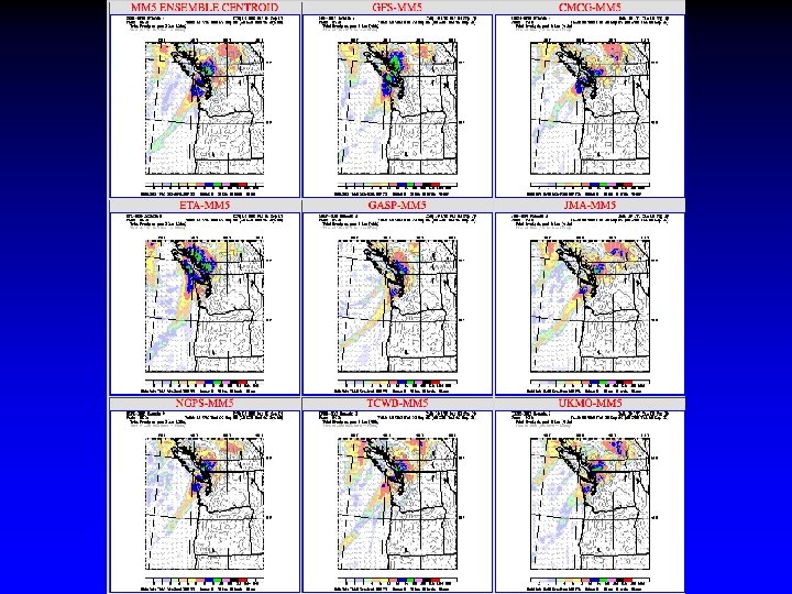
UWME – Core : 8 members, 00 and 12 Z • Each uses different synoptic scale initial and boundary conditions • All use same physics – Physics : 8 members, 00 Z only • Each uses different synoptic scale initial and boundary conditions • Each uses different physics • Each uses different SST perturbations • Each uses different land surface characteristic perturbations – Centroid, 00 and 12 Z • Average of 8 core members used for initial and boundary conditions

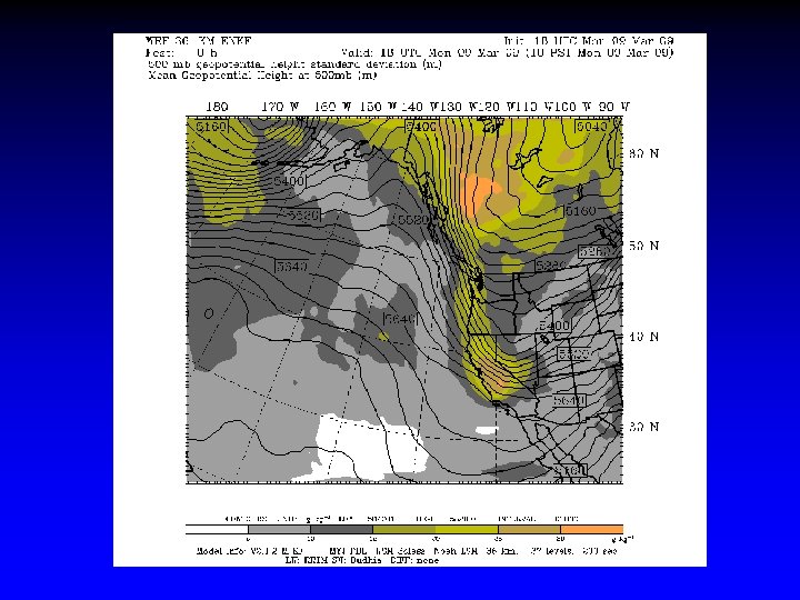
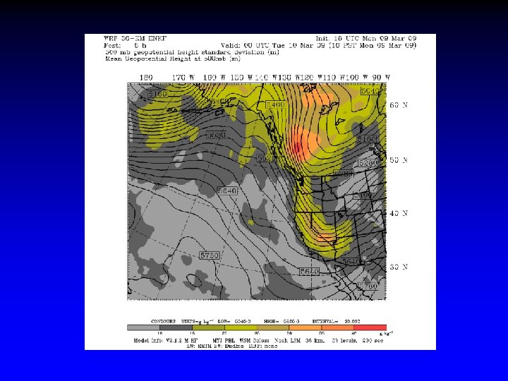
Ensemble-Based Probabilistic Products

The MURI Project • In 2000, Statistic Professor Adrian Raftery came to me with a wild idea: submit a proposal to bring together a strong interdisciplinary team to deal with mesoscale probabilistic prediction. • Include atmospheric sciences, psychologists, statisticians, web display and human factors experts.

The Muri I didn’t think it had a chance. I was wrong. It was funded and very successful.

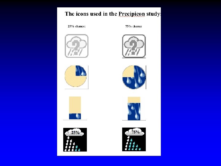
The MURI • Over five years substantial progress was made: – Successful development of Bayesian Model Averaging (BMA) postprocessing for temperature and precipitation – Development of both global and local BMA – Development of grid-based bias correction – Completion of several studies on how people use probabilistic information – Development of new probabilistic icons.

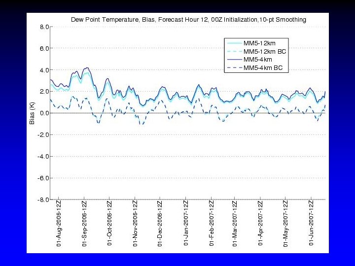
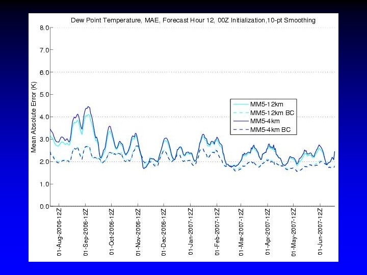
Raw 12 -h Forecast Bias-Corrected Forecast

Skill for Probability of T 2 < 0°C *UW Basic Ensemble with bias correction UW Basic Ensemble, no bias correction *UW Enhanced Ensemble with bias cor. UW Enhanced Ensemble without bias cor BSS: Brier Skill Score
")
Calibration Example-Max 2 -m Tempeature (all stations in 12 km domain)
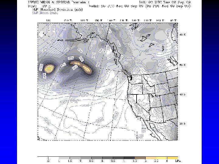
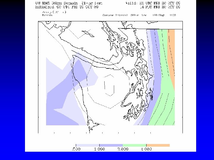
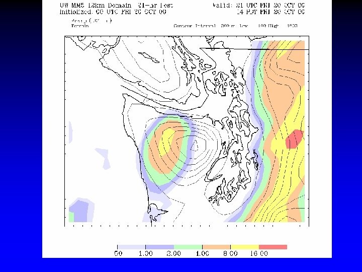
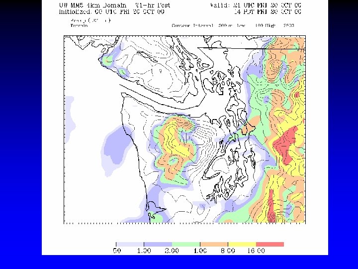
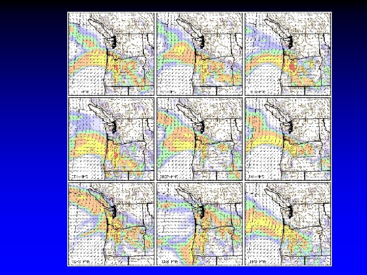
 SLP and winds")
The Thanksgiving Forecast 2001 42 h forecast (valid Thu 10 AM) SLP and winds 1: cent Verification - Reveals high uncertainty in storm track and intensity - Indicates low probability of Puget Sound wind event 2: eta 5: ngps 8: eta* 11: ngps* 3: ukmo 6: cmcg 9: ukmo* 12: cmcg* 4: tcwb 7: avn 10: tcwb* 13: avn*

Ensemble-Based Probabilistic Products

Probability Density Functio at one point Ensemble-Based Probabilistic Products

Providing forecast uncertainty information is good…. But you can have too much of a good thing…

MURI • Improvements and extensions of UWME ensembles to multi-physics • Development of BMA and probcast web sites for communication of probabilistic information. • Extensive verification and publication of a large collection of papers. • And plenty more…

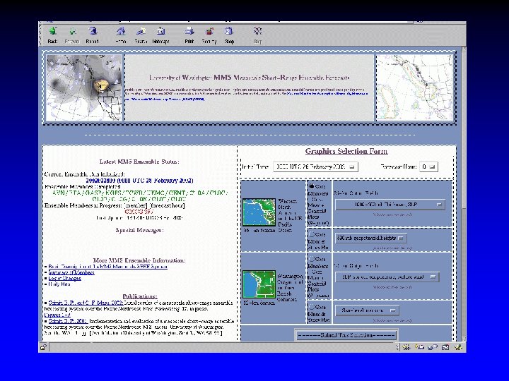
Before Probcast: The BMA Site

PROBCAST

ENSEMBLES AHEAD

The JEFS Phase • Joint AF and Navy project (at least it was supposed to be this way). UW and NCAR main contractors. • Provided support to continue development of basic parameters. • Joint project with NCAR to build a complete mesoscale forecasting system for the Air Force. • For the first few years was centered on North Korea, then SW Asia, and now the U. S.

JEFS Highlights • Under JEFS the post-processed BMA fields has been extended to wind speed and direction. Local BMA for precipitation. • Development of EMOS, a regression-based approach that produces results nearly as good as BMA. • Next steps: derived parameters (e. g. , ceiling, visibility)

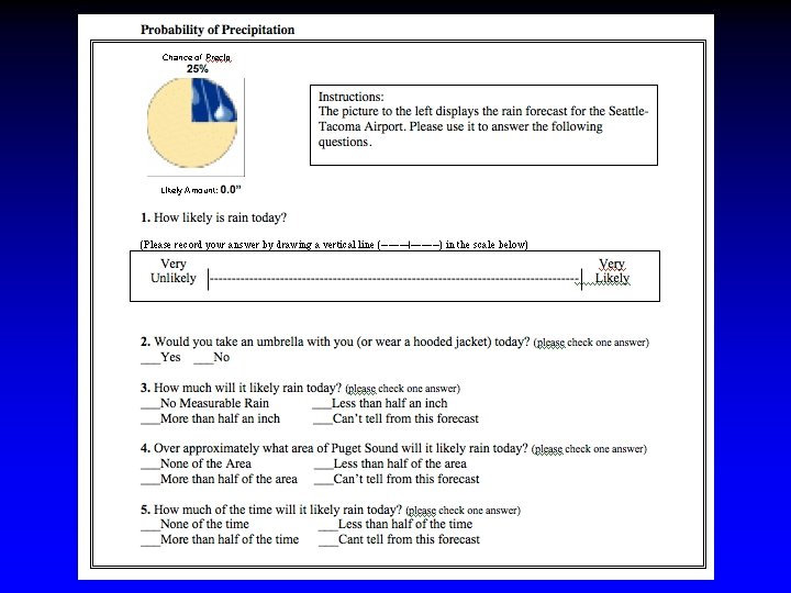
NSF Project • Currently supporting extensive series of human-subjects studies to determine how people interpret uncertainty information. • Further work on icons • Further work on probcast.

Ensemble Kalman Filter Project • Much more this afternoon. • 80 -member synoptic ensemble (36 km-12 km or 36 km) • Uses WRF model • Six-hour assimilation steps. • Experimenting with 12 and 4 km to determine value for mesoscale data assimilation-AOR in 3 D.

Big Picture • The U. S. is not where it should be regarding probabilistic prediction on the mesoscale. • Current NCEP SREF is inadequate and uncalibrated. • Substantial challenges in data poor areas for calibration and for fields like visibility that the models don’t simulate at all or simulate poorly. • A nationally organized effort to push rapidly to 4 D probabilistic capabilities is required.

Opinion • Creating sharp, reliable PDFs is only half the battle. • The hardest part is the human side, making the output accessible, useful, and compelling. We NEED the social scientists. • Probabilistic forecast information has the potential for great societal economic benefit.

The END

Brief History • Local high-resolution mesoscale NWP in the Northwest began in the mid-1990 s after a period of experimentation showed the substantial potential of small grid spacing (12 to 4 km) over terrain. • At that time NCEP was running 32 -48 km grid spacing and the Eta model clearly had difficulties in terrain.

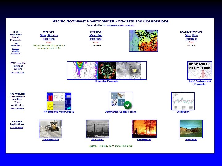
The Northwest Environmental Prediction System • Beginning in 1995, a team at the University of Washington, with the help of colleagues at Washington State University and others have built the most extensive regional weather/environmental prediction system in the U. S. • It represents a different model of how weather and environmental prediction can be accomplished.

Pacific Northwest Regional Prediction: Major Components • Real-time, operational mesoscale environmental prediction – – MM 5/WRF atmospheric model DHSVM distributed hydrological model Calgrid Air Quality Model A variety of application models (e. g. , road surface) • Real-time collection and quality control of regional observations.

Why Probcast? • We are rapidly gaining the ability to produce useful probabilistic guidance-- forecasts that are reasonably reliable and sharp. • Believe it or not, this is the easy part of the problem. • What we have not done is to design interfaces that allow users to make effective user of probabilistic output … or even convince users that they should “go probabilistic”. • The recent NRC Report on Probabilistic Prediction highlights this issue.

UW Uncertainty MURI • The DOD-sponsored UW Uncertainty MURI was designed to consider both sides of the problem: – Generation of probabilistic information-ensembles and post-processing – Display and human interface issues. • Includes UW Atmospheric Sciences, Statistics, Psychology, and Applied Physics Lab

UW Probabilistic Prediction • UW Ensemble System is based on using varying initialization and boundary conditions from differing operational analyses. • Also includes varying model physics and surface properties (e. g. , SST). • Have developed sophisticated post-processing: grid-based bias correction and Bayesian Model Averaging (BMA)--both global and local

Before Probcast: The BMA Site

UW MURI • Considerable work by Susan Joslyn and others in psychology and APL to examine how forecasters and others process forecast information and particularly probabilistic information. • One example has been their study of the interpretation of weather forecast icons.

The Winner

WRF Domains: 36 -12 -4 km

Putting it All Together • During the last year, the MURI project has attempted to create a user interface that accesses the voluminous and detailed probabilistic information produced by our system in a way that is highly accessible to lay and even professional users. • The result: PROBCAST • Available operationally at www. probcast. com

PROBCAST
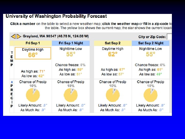

Probcast Features • Local BMA for temperature • Currently non-local BMA for precipitation (working on it) • Attempt to use probabilistic information in a way that is accessible to deterministicoriented individuals. • Can click anywhere on map to get probabilistic information for specific locations.

PROBCAST

Just the beginning • Will expand probcast to more parameters • Will improve interface from public feedback • Will be testing more icon ideas this year. • Unfortunately, MURI ends in 8 months and no replacement.

Bayesian model averaging where is the deterministic forecast from member k, is the weight associated with member k, and is the estimated density function for y given memb 61

The END

Ensemble Forecasting 48 -hour forecasts for maximum wind speeds on 7 August 2003 63

Update on the UW En. KF Mesoscale Analysis and Prediction System Brian Ancell, Clifford F. Mass, and Gregory J. Hakim The University of Washington
 Brief review of motivation for a highresolution En. KF 2) Summary of")
Outline 1) Brief review of motivation for a highresolution En. KF 2) Summary of 36 km/12 km En. KF results 3) Upgrades to En. KF system 4) Computational costs for more frequent data assimilation cycles at higher resolution

Motivation for High-resolution En. KF • Key benefit is using flow-dependent, smallscale structure during assimilation

36 -km vs. 12 -km En. KF 36 -km 12 -km SLP, 925 -mb temperature, surface winds

36 -km vs. 12 -km En. KF 36 -km 12 -km SLP, 925 -mb temperature, surface winds

36 -km vs. 12 -km En. KF 36 -km 12 -km SLP, 925 -mb temperature, surface winds

Motivation for High-resolution En. KF • Key benefit is using flow-dependent, smallscale structure during assimilation • Analysis and forecast uncertainty is a major advantage
 D 2 (12 km) D 1 (36")
En. KF Configuration D 3 (4 km) D 2 (12 km) D 1 (36 km)

En. KF Configuration • • • WRF model 38 vertical levels 80 ensemble members 6 -hour update cycle Observations: • Surface temperature, wind, altimeter • ACARS aircraft winds, temperature • Cloud-track winds • Radiosonde wind, temperature, relative humidity Half of surface obs used for assimilation, other half for

En. KF 12 km Surface Observations

En. KF 36 km vs. 12 km Wind Analys is Foreca 10% Temperatur e Improvement of 12 -km En. KF 13% 10%

Reduction of Observation Variance in 12 km En. KF Wind Analys Temperatur e Improvement using reduced observation uncertainty 5% 10%

Further Improvement After Variance Inflation, Bias Removal Wind Analys Temperatur e Improvement using inflation and bias removal 9% 3%

En. KF 12 -km vs. GFS, NAM, RUC Wind GF NA S RU M En. KF 12 C 2. 38 2. 30 m/s 2. 13 m/s 1. 85 m/s Temperatu re RMS analysis errors 2. 28 K 2. 54 K 2. 35 K 1. 67 K

En. KF System Upgrades • 4 km domain

En. KF System Upgrades 36 k m 12 k m SLP, 925 -mb temperature, surface winds 4 km

En. KF System Upgrades • 4 km domain • WRF V 2 to WRF V 3

En. KF System Upgrades • 4 km domain • WRF V 2 to WRF V 3 • Physics matched with real time GFS-WRF (changes bias and surface variance characteristics)

En. KF System Upgrades • 4 km domain • WRF V 2 to WRF V 3 • Physics matched with real time GFS-WRF (changes bias and surface variance characteristics) • Additional altimeter observations Surface observations 12 km: ~10, 000 ~5, 000 (50%) 4 km: ~5, 000 ~4, 000 (80%) Terrain check

En. KF System Timing 6 -hr cycle, 80 processors • 36 km: • 4 km assimilation: model integration: overhead: assimilation: model integration: nestdown: overhead: 12 minutes 20 minutes 5 minutes 15 minutes 240 minutes 10 minutes Total: 5 hours

En. KF System Timing 3 -hr cycle, 80 processors • 36 km: • 4 km assimilation: model integration: overhead: assimilation: model integration: nestdown: overhead: 12 minutes 10 minutes 5 minutes 120 minutes 10 minutes Total: 3 hours

En. KF System Timing 2 -hr cycle, 80 processors • 36 km: • 4 km assimilation: model integration: overhead: assimilation: model integration: nestdown: overhead: 12 minutes 7 minutes 5 minutes 15 minutes 80 minutes 10 minutes Total: 2. 3 hours

En. KF System Timing 2 -hr cycle, 160 processors • 36 km: • 4 km assimilation: model integration: overhead: assimilation: model integration: nestdown: overhead: 12 minutes 4 minutes 5 minutes 15 minutes 50 minutes 5 minutes 10 minutes Total: 1. 7 hours
- Slides: 86