MeshConnected Illiac Networks Here in mesh network nodes

Mesh-Connected Illiac Networks Here in mesh network nodes are arranged as a q-dimensional lattice. The neighboring nodes are only allowed to communicate the data in one step i. e. , each PEi is allowed to send the data to any one of PE(i+1) , PE (i-1), Pe(i+r) and PE(i-r) where r= square root N( in case of Iliac r=8). In a periodic mesh, nodes on the edge of the mesh have wrap-around connections to nodes on the other side this is also called a to raidal mesh. Mesh Metrics For a q-dimensional non-periodic lattice with kq nodes: • Network connectivity = q • Network diameter = q(k-1) • Network narrowness = k/2 • Bisection width = kq-1 • Expansion Increment = kq-1 • Edges per node = 2 q Thus we observe the output of ISk is connected to inputs of OSj where j = k-1, K+1, k-r, k+r as shown in figure.

Similarly the OSj gets input from ISk for K= j-1, j+1, j-r, j+r. The topology is formerly described by the four routing functions: • R+1(i)= (i+1) mod N => (0, 1, 2…, 14, 15) • R-1(i)= (i-1) mod N => (15, 14, …, 2, 1, 0) • R+r(i)= (i+r) mod N => (0, 4, 8, 12)(1, 5, 9, 13)(2, 6, 10, 14)(3, 7, 11, 15) • R-r(i)= (i-r) mod N => (15, 11, 7, 3)(14, 10, 6, 2)(13, 9, 5, 1)(12, 8, 4, 0) The figure given below show each PEi is connected to its four nearest neighbors in the mesh network. It is same as that used for IILiac – IV except that w had reduced it for N=16 and r=4. The index are calculated as module N. An n-dimensional mesh can be defined as an interconnection structure that has K 0 x K 1 x……. . Kn-1 nodes. where n is the number of dimensions of the network Ki is the radix of dimension i. shows an example of a 3 x 3 x 2 mesh network.

A node whose position is (i, j, k) is connected to its neighbors at dimensions i± 1, j± 1, and k± 1. Mesh architecture with wrap around connections forms a torus. A number of routing mechanisms have been used to route messages around meshes. One such routing mechanism is known as the dimension-ordering routing. Using this technique, a message is routed in one given dimension at a time, arriving at the proper coordinate in each dimension before proceeding to the next dimension. A 3 x 3 x 2 mesh network Consider, for example, a 3 D mesh. Since each node is represented by its position (i, j, k), then messages are first sent along the i dimension, then along the j dimension, and finally along the k dimension. At most two turns will be allowed and these turns will be from i to j and then from j to k. In Figure we show the route of a message sent from node S at position (0, 0, 0) to node D at position (2, 1, 1). Other routing mechanisms in meshes have been proposed. It should be noted that for a mesh interconnection network with N nodes, the longest distance traveled between any two arbitrary nodes is O(√N).

Permutation Networks Thus the permutation cycle according to routing function will be as follows: Horizontally, all PEs of all rows form a linear circular list as governed by the following two permutations, each with a single cycle of order N. The permutation cycles (a b c) (d e) stands for permutation a->b, b->c, c->a and d->e, e->d in a circular fashion with each pair of parentheses. R+1 = (0 1 2 …. N-1) R– 1 = (N-1 …. . 2 1 0). Similarly we have vertical permutation also and now by combining the two permutation each with four cycles of order four each the shift distance for example for a network of N = 16 and r = square root(16) = 4, is given as follows: R +4 = (0 4 8 12)(1 5 9 13)(2 6 10 14)(3 7 11 15) R – 4 = (12 8 4 0)(13 9 5 1)(14 10 6 2)(15 11 7 3) Mesh Redrawn

Static Interconnection Networks Static (fixed) interconnection networks are characterized by having fixed paths, unidirectional or bidirectional, between processors. Two types of static networks can be identified. These are completely connected networks (CCNs) and limited connection networks (LCNs). a) Completely Connected Networks In a completely connected network (CCN) each node is connected to all other nodes in the network. Completely connected networks guarantee fast delivery of messages from any source node to any destination node (only one link has to be traversed). q Routing of messages between nodes becomes a straightforward task. q Expensive in terms of the number of links needed for their construction (more apparent for higher values of N). q The number of links is given by N(N - 1)/2. The delay complexity of CCNs, measured in terms of the number of links traversed as messages are routed from any source to any destination is constant, that is, O(1). An example having N = 6 nodes is shown below:

b- Limited Connection Networks Limited connection networks (LCNs) do not provide a direct link from every node to every other node in the network. Instead, communications between some nodes have to be routed through other nodes in the network. The length of the path between nodes, measured in terms of the number of links that have to be traversed, is expected to be longer compared to the case of CCNs. Two other conditions seem to have been imposed by the existence of limited interconnectivity in LCNs. These are: 1 - the need for a pattern of interconnection among nodes 2 -the need for a mechanism for routing messages around the network until they reach their destinations.

A number of regular interconnection patterns have evolved over the years for LCNs. These patterns include: One dimensional topologies (a linear array network; ( simple routing mechanism but slow. ) Various 2 -D topologies : (b)ring (loop) networks; (c) two-dimensional arrays (mesh) -(nearest-neighbor mesh); (d) tree networks; star ; Systolic Array 3 -D topologies (Completely connected chordal ring ; Chordal ring ; 3 cube

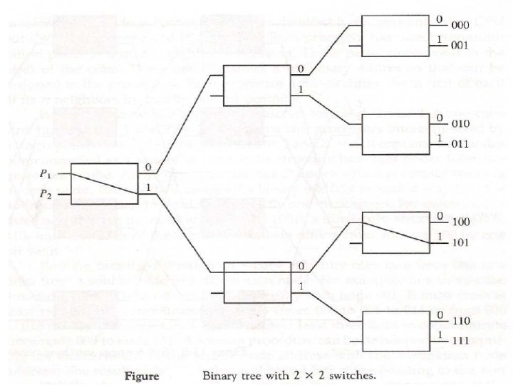
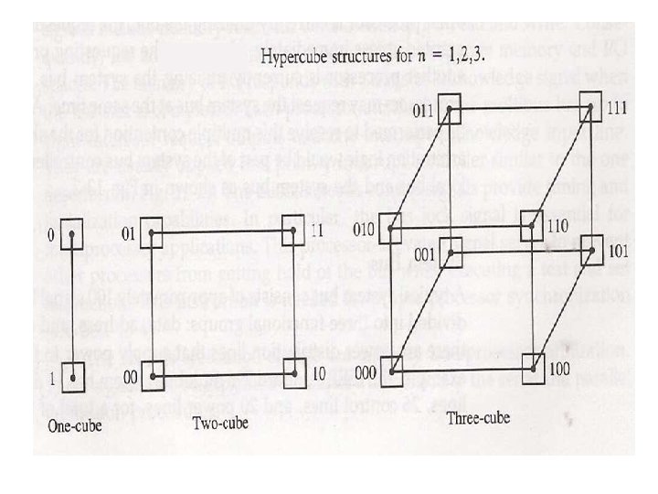
Tree Network The number of nodes (processors) in a binary tree system having k levels can be calculated as: Notice that the maximum depth of a binary tree system is, where N is the number of nodes (processors) in the network. Therefore, the network complexity is O(2 k) and the time complexity is O( log 2 N). Cube-Connected Networks Cube-connected networks are patterned after the n-cube structure. An ncube (hypercube of order n) is defined as an undirected graph having 2 n vertices labeled 0 to 2 n - 1 such that there is an edge between a given pair of vertices if and only if the binary representation of their addresses differs by one and only one bit. A 4 -cube is shown in Figure. In an n-cube, each node has a degree n. The degree of a node is defined as the number of links incident on the node. The maximum number of links a message has to traverse in order to reach its destination in an n-cube containing N = 2 n nodes is log 2 N = n links.

In an n-cube, each processor has communication links to n other processors. The route of a message originating at node i and destined for node j can be found by XOR-ing the binary address representation of i and j. If the XOR-ing operation results in a 1 in a given bit position, then the message has to be sent along the link that spans the corresponding dimension. For example, if a message is sent from source (S) node 0101 to destination (D) node 1011, then the XOR operation results in 1110. That will mean that the message will be sent only along dimensions 2, 3, and 4 (counting from right to left) in order to arrive at the destination. The order in which the message traverses the three dimensions is not important.

Torus architecture is also one of popular network topology it is extension of the mesh by having wraparound connections Figure below is a 2 D Torus This architecture of torus is a symmetric topology unlike mesh which is not. The wraparound connections reduce the torus diameter and at the same time restore the symmetry. It can be o 1 -D torus 2 -D torus 3 -D torus The torus topology is used in Cray T 3 E We can have further higher dimension circuits for example 3 -cube connected cycle. A D- dimension W-wide hypercube contains W nodes in each dimension and there is a connection to a node in each dimension. The mesh and the cube architecture actually 2 -D and 3 -D hypercube respectively. The below figure we have hypercube with dimension 4.

Routing Algorithm for Omega Network n To understand this routing algorithm, consider the 1 st stage of the Omega network to the right. n All four 1 st stage switches send 0 1 their upper outputs to switches E and G, and their lower outputs to switches F and H. 2 n Switches E and G both send their 5 3 4 outputs to switches I and J; their data can only reach the network outputs of 0, 1, 2, and 3. 6 7 A E I B F J C G K D H L n Similarly, data from switches F 0 1 2 3 4 5 6 7 and H can only reach network It should be noted that the interconnection outputs 4, 5, 6, and 7. pattern among stages follows the shuffle operation.

n Each 1 st stage switch must be BLOCKED (111) (100) set so that its upper output has a 0 E I destination with binary value 000, 1 (111) A 001, 010, or 011, i. e. having 0 in 2 B F J the first bit position of its 3 destination. 4 n Similarly, the lower output of C G K each 1 st stage switch must have a 5 6 1 in the first bit position of its D H L destination to reach outputs 100, 7 101, 110, or 111. n For example, if network input 0 has to establish a connection with network output 7 (111), then the uppermost 1 st stage switch must set itself to exchange. n If two inputs to a 1 st stage switch have the same value in the first bit position, the Omega network cannot realize this permutation. 0 1 2 3 4 5 6 7 n For example, if network input 0 has network output 4 and network input 1 has network output 7 as their destinations, then switch A is blocked since both 4 (100) and 7 (111) have bit 1 in their first bit position.

n Similarly, the 2 nd stage switch sends its upper output to switches I or K, which connect to outputs 0 (000), 1 (001), 4 (100), and 5 (101). n The lower outputs can reach switches J or L, which can access outputs 2, 3, 6, and 7 (010, 011, 110, and 111). n For the second stage, the 2 nd bit of the destination determines the setting of the switch. n Similarly, the least significant bit of the destination determines the setting of the switches in the 3 rd stage. n Since the 3 rd stage outputs are the outputs of the network, the last stage cannot block a permutation that has been routed successfully by the previous stages. 0 1 A E I B F J 4 5 C G K 4 5 6 7 D H L 6 7 2 3

Successful Omega Routing Scheme 0 111 1 011 2 001 3 110 4 000 5 101 6 010 7 100 011 000 001 0 1 000 111 101 010 100 011 010 101 100 111 110 2 3 4 5 6 7

Unsuccessful Omega Routing 0 100 1 000 BLOCK 001 100 2 101 3 011 4 111 5 001 6 010 7 110 0 1 111 011 2 3 100 BLOCK 010 101 111 110 4 5 6 7

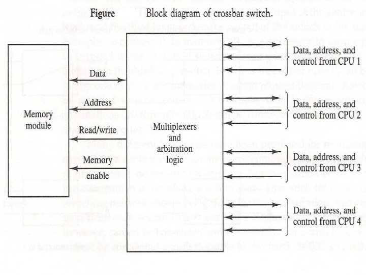
Conclusion n Interconnection networks play a central role in determining the overall performance of a multiprocessor system. And if the interconnection network cannot minimize its message latency for a particular application, then processors will frequently be forced to wait for data to arrive. The table below gives some qualitative comparisons between the various types of interconnection configurations. l Property Bus Crossbar Multistage Speed Low High Cost Low High Moderate Reliability Low High Configurability High Low Moderate Complexity Low High Moderate

21

22