MENG 3071 Chapter 2 Position Analysis All figures

MENG 3071 Chapter 2 Position Analysis All figures taken from Design of Machinery, 3 rd ed. Robert Norton 2003

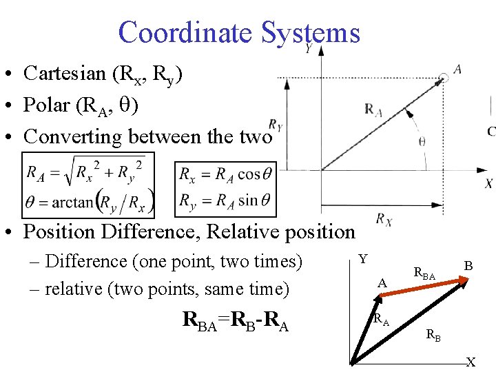
Coordinate Systems • Cartesian (Rx, Ry) • Polar (RA, q) • Converting between the two • Position Difference, Relative position – Difference (one point, two times) – relative (two points, same time) RBA=RB-RA Y A RA RBA B RB X

4. 3 Translation, Rotation, and Complex motion • Translation: keeps the same angle • Rotation: one point does not move • Complex motion: a combination of rotation and translation

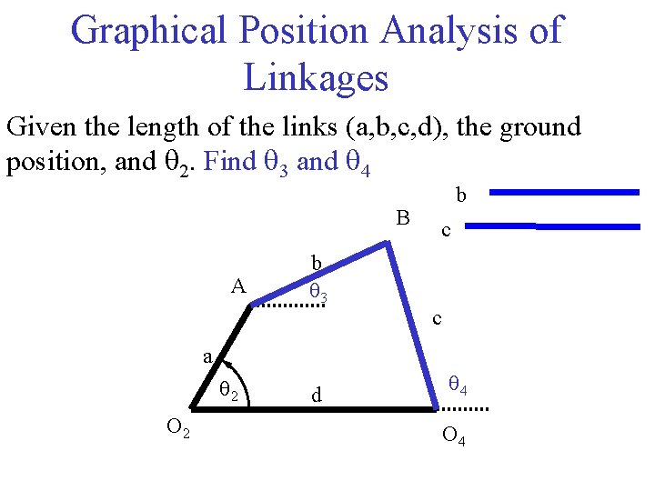
Graphical Position Analysis of Linkages Given the length of the links (a, b, c, d), the ground position, and q 2. Find q 3 and q 4 B A b q 3 b c c a q 2 O 2 d q 4 O 4

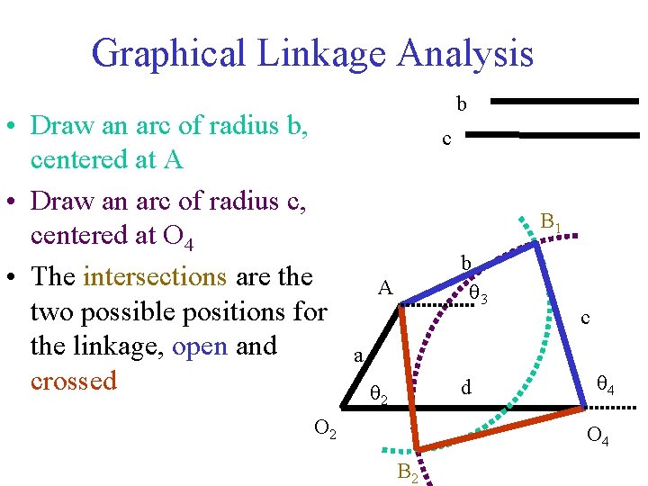
Graphical Linkage Analysis • Draw an arc of radius b, centered at A • Draw an arc of radius c, centered at O 4 • The intersections are the two possible positions for the linkage, open and crossed b c B 1 b q 3 A c a d q 2 O 2 q 4 O 4 B 2

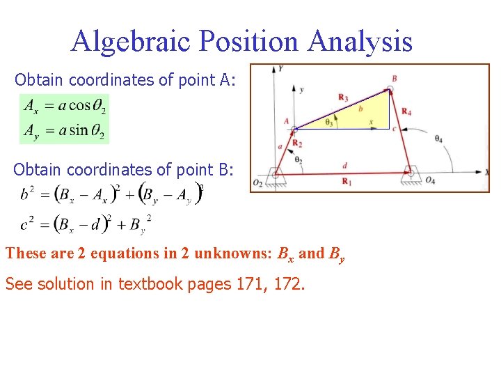
Algebraic Position Analysis Obtain coordinates of point A: Obtain coordinates of point B: These are 2 equations in 2 unknowns: Bx and By See solution in textbook pages 171, 172.

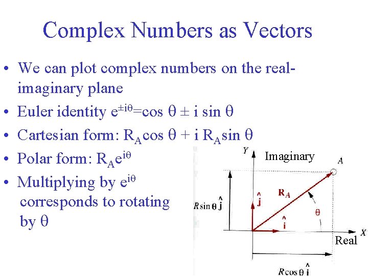
Complex Numbers as Vectors • We can plot complex numbers on the realimaginary plane • Euler identity e±iq=cos q ± i sin q • Cartesian form: RAcos q + i RAsin q Imaginary • Polar form: RAeiq • Multiplying by eiq corresponds to rotating by q Real

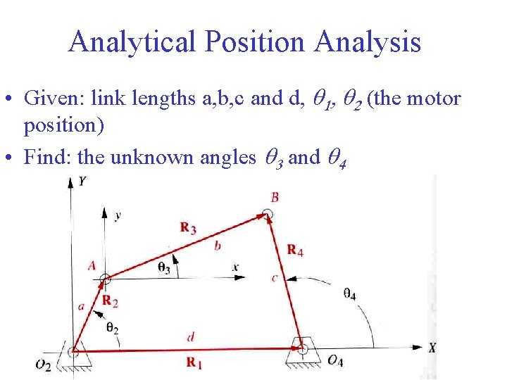
Analytical Position Analysis • Given: link lengths a, b, c and d, q 1, q 2 (the motor position) • Find: the unknown angles q 3 and q 4

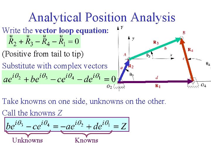
Analytical Position Analysis Write the vector loop equation: (Positive from tail to tip) Substitute with complex vectors Take knowns on one side, unknowns on the other. Call the knowns Z Unknowns Knowns

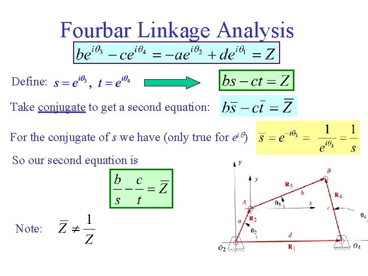
Fourbar Linkage Analysis Define: Take conjugate to get a second equation: For the conjugate of s we have (only true for eiq) So our second equation is Note:

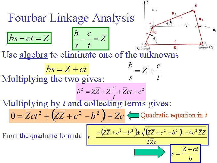
Fourbar Linkage Analysis Use algebra to eliminate one of the unknowns Multiplying the two gives: Multiplying by t and collecting terms gives: Quadratic equation in t From the quadratic formula

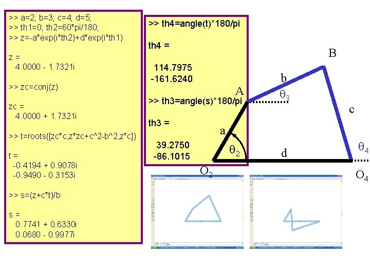
Fourbar Linkage Analysis • In MATLAB, Zc=conj(Z) t=roots([Zc*c, Z*Zc+c^2 -b^2, Z*c]) A • q 4=angle(t), q 3=angle(s) • Two solutions relate to the a open and crossed q 2 positions O 2 B 1 b q 3 d c q 4 O 4

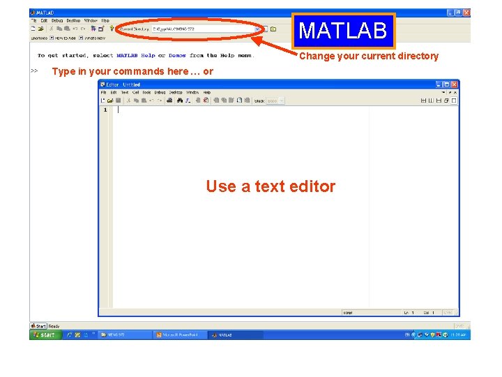
MATLAB Change your current directory Type in your commands here … or Use a text editor

>> a=2; b=3; c=4; d=5; >> th 1=0; th 2=60*pi/180; >> z=-a*exp(i*th 2)+d*exp(i*th 1) z= 4. 0000 - 1. 7321 i >> zc=conj(z) zc = 4. 0000 + 1. 7321 i >> t=roots([zc*c, z*zc+c^2 -b^2, z*c]) t= -0. 4194 + 0. 9078 i -0. 9490 - 0. 3153 i >> s=(z+c*t)/b s= 0. 7741 + 0. 6330 i 0. 0680 - 0. 9977 i >> th 4=angle(t)*180/pi th 4 = B 114. 7975 -161. 6240 A >> th 3=angle(s)*180/pi th 3 = b q 3 c a 39. 2750 -86. 1015 q 2 O 2 d q 4 O 4

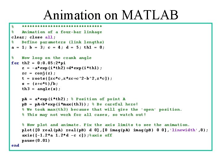
Animation on MATLAB % **************** % Animation of a four-bar linkage clear; close all; % Define parameters (link lengths) a = 1; b = 3; c = 4; d = 5; th 1 = 0; % Now loop on the crank angle for th 2 = 0: 0. 05: 2*pi z = -a*exp(i*th 2)+d*exp(i*th 1); zc = conj(z); t = roots([zc*c, z*zc+c^2 -b^2, z*c]); s = (z+c*t)/b; th 3 = angle(s); p. A = a*exp(i*th 2); % Position of point A p. B = p. A+b*exp(i*max(th 3)); % Be careful here! % We took max(th 3) because that will give the 'open' position. % This may not work for all cases, so watch out! % Now plot and animate. Fix the axis limits to see the animation. plot([0 real(p. A) real(p. B) d 0], [0 imag(p. A) imag(p. B) 0 0], 'linewidth', 8); axis([-1. 2*a 1. 2*d -c c]); %axis off pause(0. 01) end

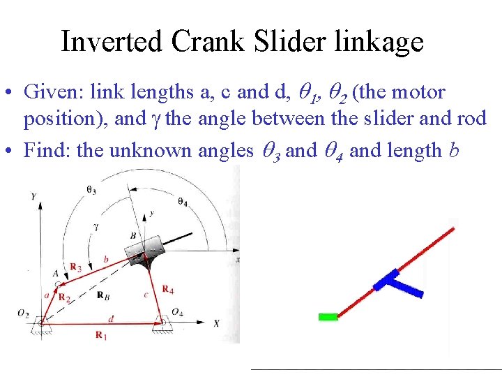
Inverted Crank Slider linkage • Given: link lengths a, c and d, q 1, q 2 (the motor position), and g the angle between the slider and rod • Find: the unknown angles q 3 and q 4 and length b

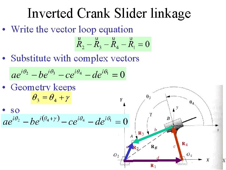
Inverted Crank Slider linkage • Write the vector loop equation • Substitute with complex vectors • Geometry keeps • so

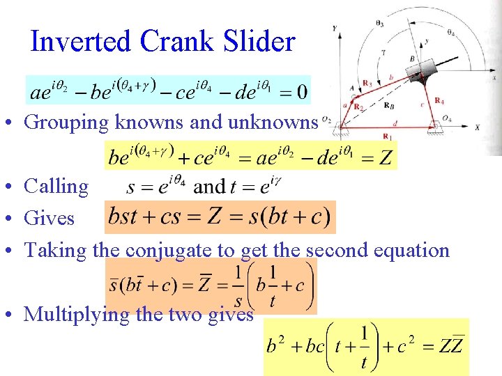
Inverted Crank Slider • Grouping knowns and unknowns • Calling • Gives • Taking the conjugate to get the second equation • Multiplying the two gives

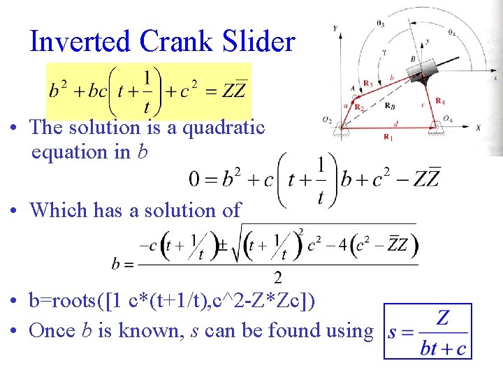
Inverted Crank Slider • The solution is a quadratic equation in b • Which has a solution of • b=roots([1 c*(t+1/t), c^2 -Z*Zc]) • Once b is known, s can be found using

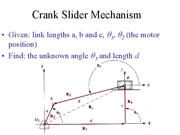
Crank Slider Mechanism • Given: link lengths a, b and c, q 1, q 2 (the motor position) • Find: the unknown angle q 3 and length d

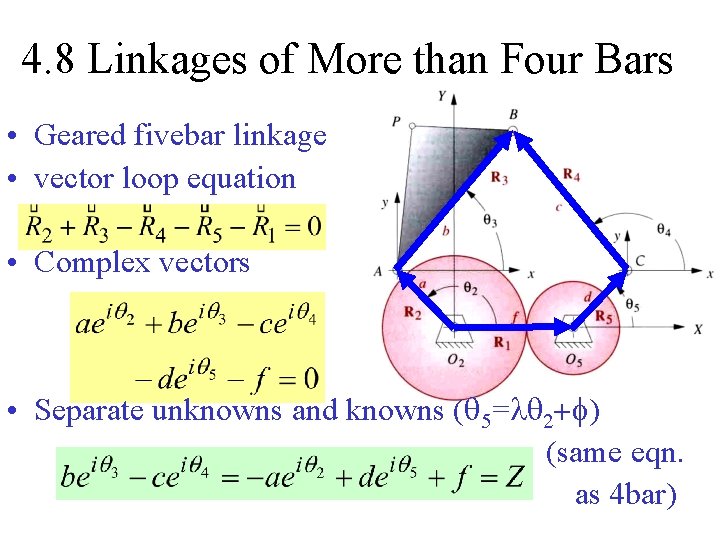
4. 8 Linkages of More than Four Bars • Geared fivebar linkage • vector loop equation • Complex vectors • Separate unknowns and knowns (q 5=lq 2+f) (same eqn. as 4 bar)

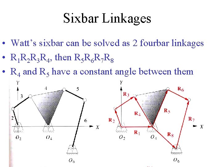
Sixbar Linkages • Watt’s sixbar can be solved as 2 fourbar linkages • R 1 R 2 R 3 R 4, then R 5 R 6 R 7 R 8 • R 4 and R 5 have a constant angle between them

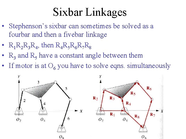
Sixbar Linkages • Stephenson’s sixbar can sometimes be solved as a fourbar and then a fivebar linkage • R 1 R 2 R 3 R 4, then R 4 R 5 R 6 R 7 R 8 • R 3 and R 5 have a constant angle between them • If motor is at O 6 you have to solve eqns. simultaneously

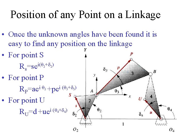
Position of any Point on a Linkage • Once the unknown angles have been found it is easy to find any position on the linkage • For point S Rs=sei(q +d ) • For point P RP=aei q +pei (q +d ) • For point U RU=d +uei (q +d ) 2 2 2 3 4 4 3

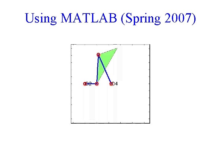
Using MATLAB (Spring 2007)

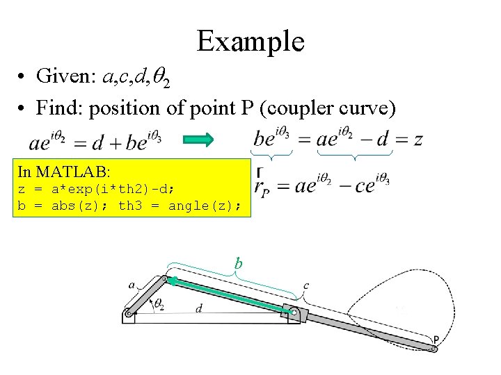
Example • Given: a, c, d, q 2 • Find: position of point P (coupler curve) In MATLAB: z = a*exp(i*th 2)-d; b = abs(z); th 3 = angle(z); b

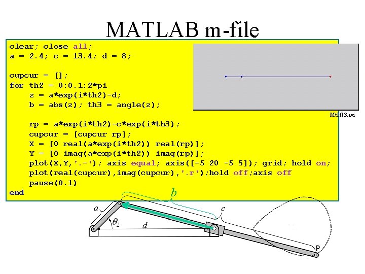
MATLAB m-file clear; close all; a = 2. 4; c = 13. 4; d = 8; cupcur = []; for th 2 = 0: 0. 1: 2*pi z = a*exp(i*th 2)-d; b = abs(z); th 3 = angle(z); Mt 1 f 13. avi rp = a*exp(i*th 2)-c*exp(i*th 3); cupcur = [cupcur rp]; X = [0 real(a*exp(i*th 2)) real(rp)]; Y = [0 imag(a*exp(i*th 2)) imag(rp)]; plot(X, Y, '. -'); axis equal; axis([-5 20 -5 5]); grid; hold on; plot(real(cupcur), imag(cupcur), '. r'); hold off; axis off pause(0. 1) end b

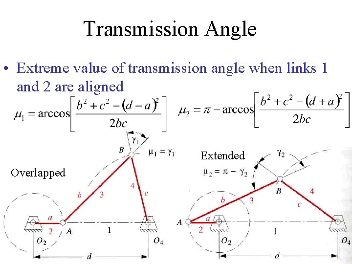
Transmission Angle • Extreme value of transmission angle when links 1 and 2 are aligned Extended Overlapped

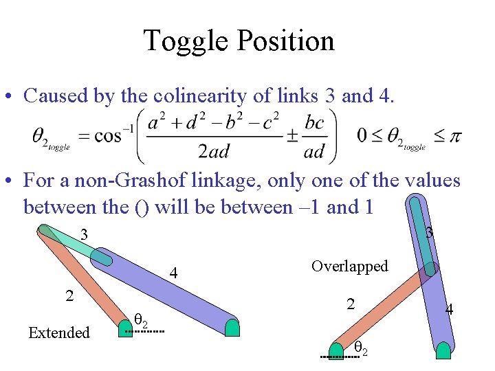
Toggle Position • Caused by the colinearity of links 3 and 4. • For a non-Grashof linkage, only one of the values between the () will be between – 1 and 1 3 3 4 2 Extended q 2 Overlapped 2 q 2 4