Mendelian Randomization Genes as Instrumental Variables David Evans

Mendelian Randomization: Genes as Instrumental Variables David Evans University of Queensland
? • Examples of MR in research")
This Session • What is Mendelian Randomization (MR)? • Examples of MR in research • Some ideas • Using R to perform MR

Some Criticisms of GWA Studies… • So you have a new GWAS hit for a disease… so what!? • You can’t change people’s genotypes (at least not yet) • You can however modify people’s environments… • Mendelian Randomization is a method of using genetics to inform us about associations in traditional observational epidemiology

RCTs are the Gold Standard in Inferring Causality RANDOMISED CONTROLLED TRIAL RANDOMISATION METHOD EXPOSED: INTERVENTION CONTROL: NO INTERVENTION CONFOUNDERS EQUAL BETWEEN GROUPS OUTCOMES COMPARED BETWEEN GROUPS

Observational Studies • RCTs are expensive and not always ethical or practically feasible • Association between environmental exposures and disease can be assessed by observational epidemiological studies like case-control studies or cohort studies • The interpretation of these studies in terms of causality is problematic

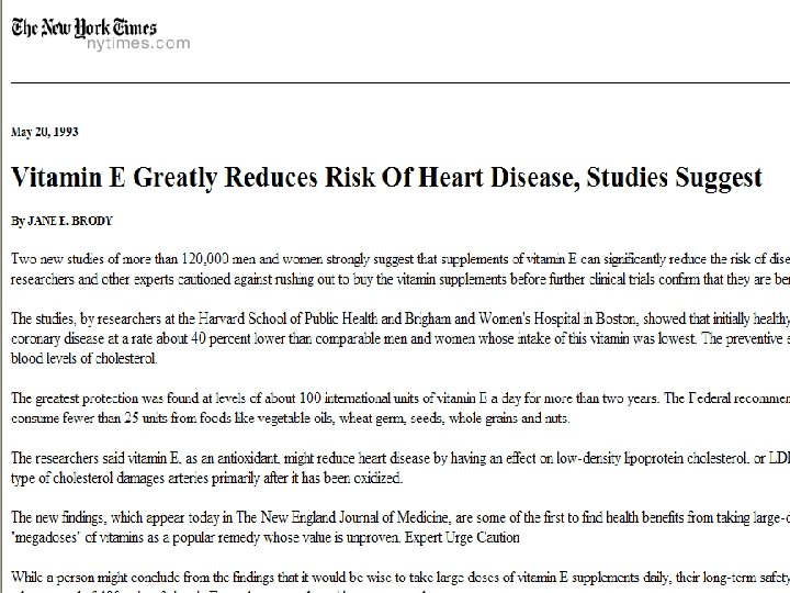
CHD risk according to duration of current Vitamin E supplement use compared to no use RR Rimm et al NEJM 1993; 328: 1450 -6


Percent Use of vitamin supplements by US adults, 1987 -2000 Source: Millen AE, Journal of American Dietetic Assoc 2004; 104: 942 -950

Vitamin E levels and risk factors: Women’s Heart Health Study Childhood SES Manual social class No car access State pension only Smoker Daily alcohol Exercise Low fat diet Obese Height Leg length Lawlor et al, Lancet 2004

Vitamin E supplement use and risk of Coronary Heart Disease 1. 0 Stampfer et al NEJM 1993; 328: 144 -9; Rimm et al NEJM 1993; 328: 1450 -6; Eidelman et al Arch Intern Med 2004; 164: 1552 -6

“Well, so much for antioxidants. ”

Classic limitations to “observational” science • Confounding • Reverse Causation • Bias

An Alternative to RCTs: Mendelian randomization In genetic association studies the laws of Mendelian genetics imply that comparison of groups of individuals defined by genotype should only differ with respect to the locus under study (and closely related loci in linkage disequilibrium with the locus under study) Genotypes can proxy for some modifiable risk factors, and there should be no confounding of genotype by behavioural, socioeconomic or physiological factors (excepting those influenced by alleles at closely proximate loci or due to population stratification) Mendel in 1862

Mendelian randomisation and RCTs MENDELIAN RANDOMISATION RANDOM SEGREGATION OF ALLELES EXPOSED: FUNCTIONAL ALLELLES CONTROL: NULL ALLELLES CONFOUNDERS EQUAL BETWEEN GROUPS OUTCOMES COMPARED BETWEEN GROUPS RANDOMISED CONTROLLED TRIAL RANDOMISATION METHOD EXPOSED: INTERVENTION CONTROL: NO INTERVENTION CONFOUNDERS EQUAL BETWEEN GROUPS OUTCOMES COMPARED BETWEEN GROUPS

Assumptions of Mendelian randomisation analysis U Z X • Z associated with X • Z is independent of U • Z is independent of Y given U and X Y

Examples – using instruments for adiposity U Z FTO Adiposity X Y

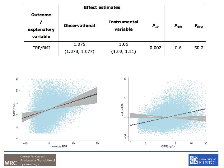
Examples – using instruments for adiposity U FTO Adiposity Traits of metabolism CRP/BMI

In a Nutshell • If adiposity DOES NOT causally affect metabolic traits, then the FTO variant should NOT be related to these metabolic traits • If adiposity causally affects metabolic traits, then the FTO variant should also be related to these metabolic traits • In this situation, the causal effect of adiposity can be estimated using an “instrumental variables analysis” as fitted by two stage least squares

Do intermediate metabolic traits differ as one would expect given a FTO-BMI effect? Given the per allele FTO effect of ~0. 1 SD and known observational estimates one can derive an expected, per allele, effect on metabolic traits Phenotype Expected Change Observed Change (BMI adjusted) Fasting insulin 0. 038 (0. 033, 0. 043) 0. 039 (0. 013, 0. 064) -0. 005 (-0. 027, 0. 018) Fasting Glucose 0. 018 (0. 014, 0. 021) 0. 024 (0. 001, 0. 048) 0. 006 (-0. 017, 0. 029) -0. 032 (-0. 057, -0. 008) -0. 004 (-0. 027, 0. 019) Fasting HDL -0. 026 (-0. 029, -0. 023) … N~12, 000 samples of European ancestry

Examples – using instruments for adiposity U FTO Adiposity Traits of metabolism CRP

Bidirectional MR
 is a biomarker of inflammation • It")
CRP and BMI • C-Reactive Protein (CRP) is a biomarker of inflammation • It is associated with BMI, metabolic syndrome, CHD and a number of other diseases • It is unclear whether these observational relationships are causal or due to confounding or reverse causality • This question is important from the perspective of drug development

“Bi-directional Mendelian Randomization” ? ? ?

Informative Interactions
, doi:")
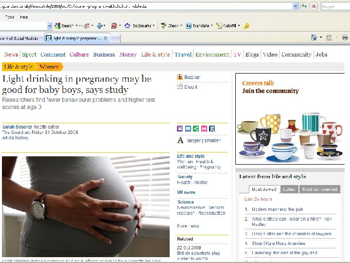
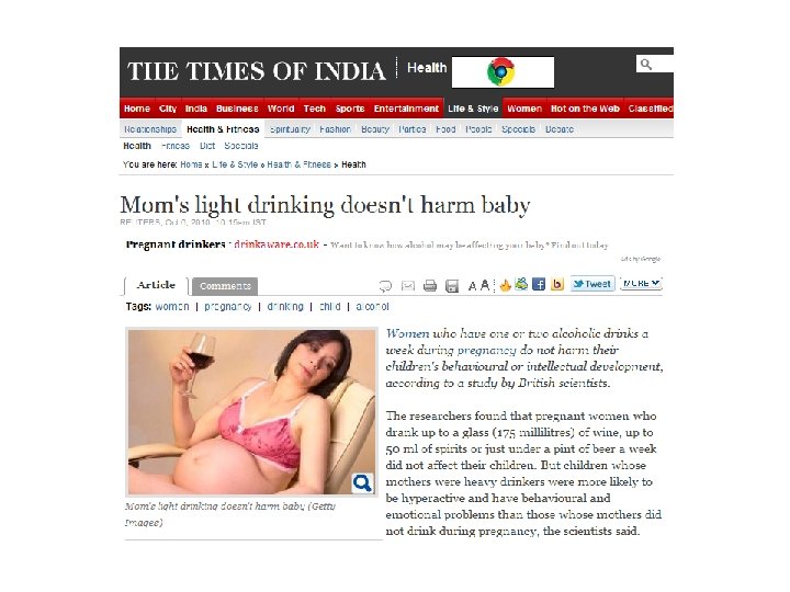
Kelly Y, Sacker A, Gray R et al. J Epidemiol Community Health (2010), doi: 10. 1136/jech. 2009. 103002
, doi:")
Kelly Y, Sacker A, Gray R et al. J Epidemiol Community Health (2010), doi: 10. 1136/jech. 2009. 103002
, doi:")
Kelly Y, Sacker A, Gray R et al. J Epidemiol Community Health (2010), doi: 10. 1136/jech. 2009. 103002

Maternal Alcohol Dehydrogenase and Offspring IQ
 risk allele score in offspring and offspring IQ, stratified")
IQ Change Alcohol dehydrogenase (ADH) risk allele score in offspring and offspring IQ, stratified by maternal alcohol intake during pregnancy Women not drinking in pregnancy All women Women drinking during pregnancy P value for interaction of risk allele score and drinking during pregnancy equals 0. 009 Lewis S et al, PLo. S One Nov 2012.

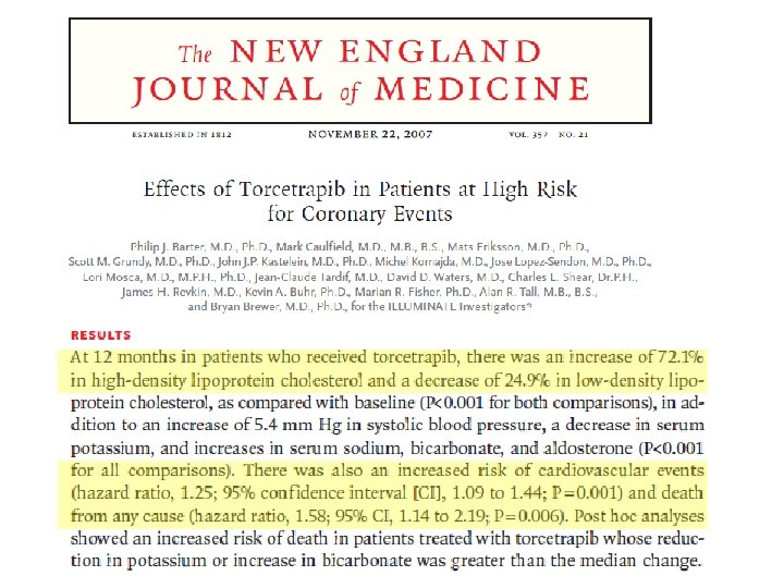
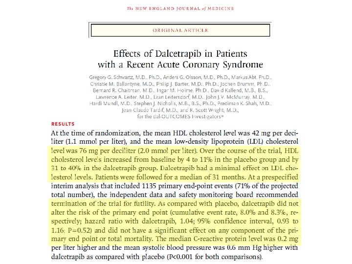
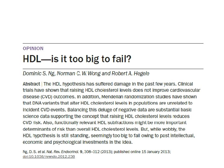
 LDL-C HDL-C 302")
Association of LDL-C, HDL-C, and risk for coronary heart disease (CHD) LDL-C HDL-C 302 K participants in 68 prospective studies Emerging Risk Factors Collaboration, JAMA 2009

LDL and CHD Risk Ference et al, JACC 2012

HDL: endothelial lipase Asn 396 Ser • • 2. 6% of population carry Serine allele higher HDL-C No effect on other lipid fractions No effect on other MI risk factors Edmondson, J Clin Invest

LIPG N 396 S and plasma HDL-C HDL Difference 396 S carriers have 5. 5 mg/dl higher HDL-C P<10 -8

After testing in 116, 320 people, summary OR for LIPG Asn 396 Ser is 0. 99

Individuals who carry the HDL-boosting variant have the same risk for heart attack as those who do not carry the variant
 Stat")
Using Multiple Genetic Variants as Instruments • Allelic scores Palmer et al (2011) Stat Method Res • Testing multiple variants individually
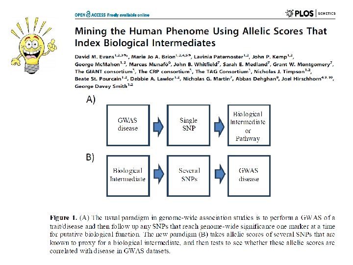

Mining the Phenome Using Allelic Scores • Could be applied to hundreds of thousands of molecular phenotypes simultaneously (gene expression, methylation, metabolomics etc)

Limitations to Mendelian Randomisation 1 - Pleiotropy 2 - Population stratification 3 - Canalisation 4 - Power (also “weak instrument bias”) 5 - The existence of instruments

Mendelian Randomization in R • There is a positive observational association between body mass index (BMI) and bone mineral density (BMD) • It is unclear whether this represents a causal relationship • We will use two stage least squares as implemented in R to address this question and estimate the causal effect of BMI on BMD

Fitting in R - Datafile BMI. 371031158022524 -. 77975167453452 -. 697738302042461. . . BMD. 860471934. 862923791. 86130172 BMI_SCORE 0. 0554687 0. 06125 0. 0684375
 #Load BMI and BMD Data x <- read. table(file=\"BMI_BMD_known. txt\",")
Fitting in R library(sem) #Load BMI and BMD Data x <- read. table(file="BMI_BMD_known. txt", header=TRUE, na. strings=-9) #Observational regression of BMD on BMI print("Observational regression of BMD on BMI") summary(lm(x$BMD ~ x$BMI)) #Regression of BMI on BMI score – Check Instrument Strength print("Regression of BMI on BMI score") summary(lm(x$BMI ~ x$BMI_SCORE)) #Perform two stage least squares analysis print("Two stage least squares analysis of BMD on BMI score") summary(tsls(x$BMD ~ x$BMI, ~ x$BMI_SCORE))
 summary(lm(x$BMD")
COMMAND: #Observational regression of BMD on BMI print("Observational regression of BMD on BMI") summary(lm(x$BMD ~ x$BMI)) OUTPUT: [1] "Observational regression of BMD on BMI" Call: lm(formula = x$BMD ~ x$BMI) Coefficients: Estimate Std. Error (Intercept) 0. 9020479 0. 0006254 x$BMI 0. 0195233 0. 0006458 t value 1442. 38 30. 23 Pr(>|t|) <2 e-16 ***

COMMAND: #Regression of BMI on BMI score – Check Instrument Strength print("Regression of BMI on BMI score") summary(lm(x$BMI ~ x$BMI_SCORE)) OUTPUT: [1] "Regression of BMI on BMI score" Call: lm(formula = x$BMI ~ x$BMI_SCORE) Coefficients: (Intercept) x$BMI_SCORE Estimate Std. Error -1. 30067 0. 09708 20. 56254 1. 53438 t value -13. 4 Pr(>|t|) <2 e-16 *** Residual standard error: 0. 9532 on 5552 degrees of freedom Multiple R-squared: 0. 03133, Adjusted R-squared: 0. 03116 F-statistic: 179. 6 on 1 and 5552 DF, p-value: < 2. 2 e-16

COMMAND: #Perform two stage least squares analysis print("Two stage least squares analysis of BMD on BMI score") summary(tsls(x$BMD ~ x$BMI, ~ x$BMI_SCORE)) OUTPUT: [1] "Two stage least squares analysis of BMD on BMI score" 2 SLS Estimates Model Formula: x$BMD ~ x$BMI Instruments: ~x$BMI_SCORE Estimate Std. Error t value Pr(>|t|) (Intercept) 0. 90199 0. 0006302 1431. 368 0. 000 e+00 x$BMI 0. 01442 0. 0036687 3. 931 8. 551 e-05

Acknowledgments • George Davey Smith • Nic Timpson • Sek Kathiresan
- Slides: 55