Meet the Neurons Models of the brain hardware

A Real Neuron The Neuron

Neuron Models

Mcculloch-Pitts 1940’s • • • Y = f(next) = f( S wi xi + b) Wi are weights Xi are inputs B is a bias term F() is activation function – F = 1 if next >= 0 else -1

Activation Functions Modified Mcculloch-pitts • The function shown before is a threshold function • Tanh function • Logistic

Human Brain • Neuron Speed - 10 -3 seconds per operation • Brain weights about 3 pounds and at rest consumes 20% of the bodies oxygen. • Estimates place neuron count at 1012 to 1014 • Connectivity can be 10, 000

What is the capacity of the brain? • Estimate the MIPS of a brain • Estimate the MIPS needed by a computer to simulate the brain

Structure • The cortex is estimated to be 6 layers • The brain does recognition type computations is 100 -200 milliseconds • The brain clearly uses some specialized structures.

Two Approaches • Artificial Neural Nets • Biologically inspired Neural Nets

Survey of Artificial Neural Networks

Alan Turing’s Idea X 1 X 2 0 1 0 0 1 1 1 0

Turing (Cont) B type link

B type link

Biowall

The Perceptron Rosenblatt - 1950’s • Linear classifiers • Mcculloch-pitts neurons: x 1 1 x 2 2 xn m y 1 y 2 ym

Perceptron Operation • • Unit Step Function Activation Y = Step{S wi * xi} Learning rule W(t+1) = W(t) + (a * xi * e) – a is a constant – e is error

A Example • Single Neuron trained for logical or Example taken from “Artificial Intelligence Illuminated” by Be Coppin Step one random assignments of the weights on each input w 1 = -0. 2 and w 2 = +0. 4 Set a to 0. 2 (a guess!)

Ex (cont) • Training Set: 0 0 1 1 1 0 1 1

Ex (cont) • X 1 = 0, x 2 = 0 we expect 0 • Y = Step{S wi * xi} • = Step {(0 * -0. 2) + (o * 0. 4)} = 0 • E = 0 no error! -> no change to weights • Try x 1 = 0 and x 2 = 1 expect 1

Ex (cont) • • Answer Y = 1 -> no error But X 1 = 0 and X 2 = 0 Y = 0 error is 1 ( e = expect – actual) W 1 = -0. 2 + (0. 2 * 1) = 0 W 2 = 0. 4 Now do the last case – correct no adj. Required!

Ex (cont) • We call this an epoch – one pass of the training data. • If we keep going, it takes three epoch to reach a trained network. – W 1 = 0. 2 and w 2 = 0. 4

Perceptron Capabilities • Rosenblatt modeled systems with a visual input. • Perceptrons are linear classifiers – In a two dimensional system this means separate sets of points with a line dividing the plane

Multi-layer Feed Forward x 1 1 1 x 2 2 2 xn m m

Back Propagation • Present input then measure desired vs. . Actual outputs • Correct weights by back propagating error though net • Hidden layers are corrected in proportion to the weight they provide to output stage. • Need a constant, used to prevent rapid training

Back Propagation Training • Use the sigmoid activation function – s(x) = 1 / (1 + e –x) • This has a derivative: – d s(x) / dx = s(x)(1 - s(x)) • Given the eq. for each neuron: – Xj = Sxi * wi, j – qj – Yj = s(Xj)

Cont • Error at output layer is – ek = dk – yk • Error Gradient – dk = dyk/dxk ek Note should be a partial derivative – dk = yk (1 – yk) ek

cont • W(t+1) = W(t) + a * x * d • Hidden layer nodes (back propagate the error) – dj = yj (1 -yj) Swjk dk

Improve Back Propagation • Add momentum. • DWij(t) = a * xi * dj + b Dwij(t-1)

Recurrent Networks D D D

Recurrent with Hidden Neurons D D

Properties • Memory • But can have stability issues

Training Vs. Learning • Learning is ‘self directed” • Training is externally controlled – Set of pairs of inputs and desired outputs

Learning Vs. Training • Hebbian learning: – Strengthen connections that are fired at same time • Training: – Back propagation – Hopfield networks – Boltzman machines

Hopfield Networks • • Single layer Each neuron receives and input Each neuron has connections to all others Training by “clamping” and adjusting weights

Hopfield Details • Activation function is Sign(x) • Sign(x) = +1 if X>0, -1 other wise • Hamming Distance

Boltzman Machines • Change f() in Mc. Culloch-Pitts to be probabilistic • The energy gap between 0 and 1 outputs is related to a “temperature” • pk = 1 / [ 1 + e t] t = -DEk / T • Learning: – Hold inputs and outputs according to training data – Anneal temperature while adjusting weights

Kohonen Maps • Self organizing feature map • Winner take all learning algorithm • Clusters data • Two layers input and cluster

Kohonen Operation • Feed a input vector in – Neuron ath matches best is the winner. • Euclidean Distance between vectors with weights w – Di = SQRT(S(wij-xj)2 ) – Smallest distance wins! And is updated – wij = wij + a(xj-wij )

Kohonen Operation(cont) • Sometimes a neighborhood around winner is also updated.

Kohonen Example • Two inputs and 3 x 3 cluster layer: x 2 x 1

Ex (cont) • The training will cluster the data and also the distance between clusters can be measured. • The example is very simple! Usually use a bigger map!

PDP - an turning point • Parallel Distributed Processing (1985) • Properties: – Learning similar to observed human behavior – Knowledge is distributed! – Robust

Connectionism • Superposition principle – Distributed “knowledge representation” • Separation of process and “knowledge representation” • Knowledge representation is not symbolic in the same sense as symbolic AI!

Example 1 • • Face recognition – Gary Cottrell Input a 64 x 64 grid Hidden layer 80 neurons Output layer 8 neurons – face yes, no, 2 bits for gender and 5 bits for name • Results: – Recognized the input set – 100% – Face / no-face on new faces – 100% – Male / female determination on new faces – 81%

Example 2 • SRI worked on a net to spot tanks • Used pictures of tanks and non-tanks • Pictures were both exposed and hidden vehicles! • When it worked, exposed it to new pictures • It failed! Why?

Example 3 The nature of Sub-symbolic • Categorize words by lexical type based on word order (Elman 1991)

Elman’s Network output Hidden Layer Input Context Units

Training • Set build from sample sentences – 29 words – 10, 000 two and three word sentences – Training sample is input word and following word pair • No unique answer – output is a set of words • Analysis of the trained network – – No symbol in the hidden layer corresponding to words or word pairs!!

Analysis of Networks – How? • Problem – Neural systems seem very unpricipled • Principle Component Analysis. • De-compile nets to rules

Guido Bologna Symbolic Rule Extraction • How is this possible? • Given a single neuron of N inputs • The neuron’s input form an N dimensional space • The output divides the space by a hyperplane

(cont) • The previous statement means we could write a function or rule for the neuron. • Now using the weights between the output layer and the hidden layer – select hidden layer neurons that drive the desired output. • Input to these hidden layers form rule anticedents.

(cont) • Finally use boolean algebra to form a logical rule

Other techniques • There are some very math heavy methods – Eigen Tensor analysis

Connectionisms challenge • Fodor’s Language of the Mind • Folk Psychology – mind states and our tags for them • How does the brain get to these? • Marr’s type 1 theory – competence with out explanations • See Associative Engines by Andy Clark for more!

How about some reality?

Pulsed Systems • Real neurons pulse! • Pulsed neurons have computing power over level

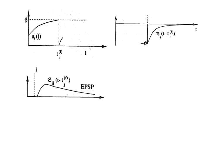
Spike Response Model • Variable ui describes the internal state • Firing times are: – Fi = {ti(f) ; i< f < n} = {t | ui(t) = threshold } – After a spike, the state variable's value is lowered • Inputs – ui= S wij eij(t - tj(f))

Models • Full Models – Simulate continuous functions – Can integrate other factors • Currents other than dendrite • Chemical states • Spike Models – Simplify and treat output as an impulse

Computational Power • Spiked Neurons Power – All the neurons are Turing Computable – Can do some things cheaper in neuron count

Encoding Problem • How does the human brain use the spike trains? • Rate Coding – Spike density – Rate over population • Pulse Coding – Time to first spike – Phase – Correlation

Where Next? • Build a brain model! • Analyze the operation of real brains • Symbolic – Neural Bridge