Median filter The median filter is used for

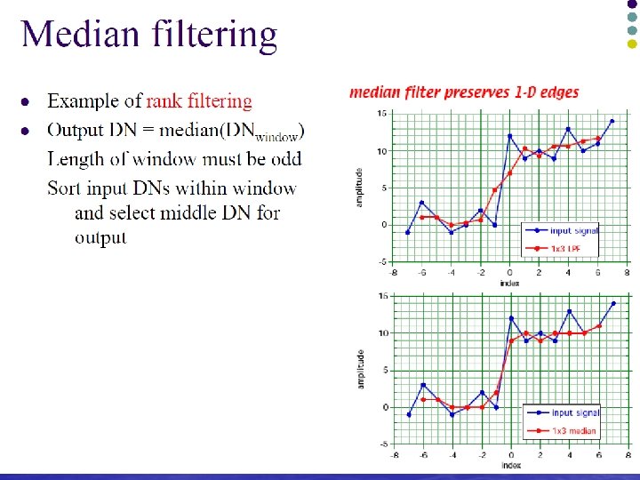
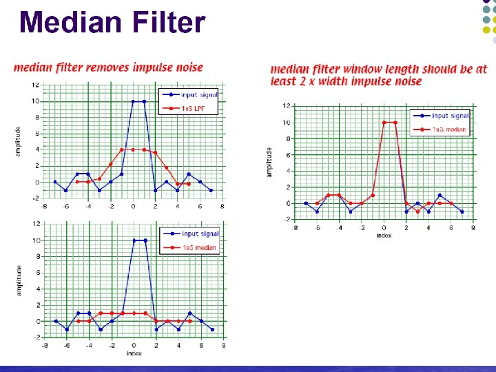
Median filter

The median filter is used for removing noise. It can remove isolated impulsive noise and at the same time it preserves the edges and other structures in the image. Contrary to average filtering it does not smooth the edges.

Unlike the mean filter, the median filter is non -linear. This means that for two images A(x) and B(x):

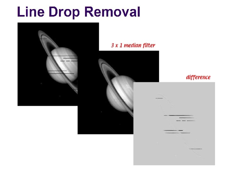
Removal of Line Artifacts by Median Filtering

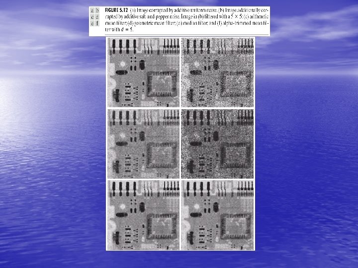
The original image. b) Original image corrupted by salt and pepper noise (p=5 % that a bit is flipped. c) After smoothing with a 3 x 3 filter most of the noise has been eliminated.

d) If we smooth the image with a larger median filter, e. g. 7 x 7, all the noise pixels disappear. e) Alternatively, we can pass a 3 x 3 filter over the image 3 times in order to remove the noise with less loss of detail.

Salt and pepper noise (5 %) Salt and pepper noise (20 %) Smoothed by 3 x 3 window

Salt and pepper noise (5 %) Salt and pepper noise (20 %) Median filtered by 3 x 3 window

Example 5. 3 Iteratively applying median filter to an image corrupted by impulse noise.

Median Filter Image. J Plugin Get Image width + height, and Make copy of image Array to store pixels to be filtered. Good data structure in which to find median Copy pixels within filter region into array Sort pixels within filter using java utility Arrays. sort( ) Middle (k) element of sorted array assumed to be middle. Return as median

Weighted Median Filter Color assigned by median filter determined by colors of “the majority” of pixels within the filter region Considered robust since single high or low value cannot influence result (unlike linear average) Median filter assigns weights (number of “votes”) to filter positions To compute result, each pixel value within filter region is inserted W(i, j) times to create extended pixel vector Extended pixel vector then sorted and median returned

Weighted Median Filter Pixels within filter region Insert each pixel within filter region W(I, j) times into extended pixel vector Sort extended pixel vector and return median Weight matrix Note: assigning weight to center pixel larger than sum of all other pixel weights inhibits any filter effect (center pixel always carries majority)!!

Alpha-trimmed mean filter is windowed filter of nonlinear class, by its nature is hybrid of the mean and median filters. The basic idea behind filter is for any element of the signal (image) look at its neighborhood, discard the most atypical elements and calculate mean value using the rest of them.

Alpha-Trimmed Mean Filter • Combining the advantages of mean filter and order-statistics filter. – Suppose delete d/2 lowest and d/2 highest gray-level value in the neighborhood of Sxy and average the remaining mn-d pixel, denoted by gr(s, t). where d=0 ~ mn-1

Adaptive Filter • Filters whose behavior changes based • on statistical characteristics of the image. Two adaptive filters are considered: (1) Adaptive, local noise reduction filter. (2) Adaptive median filter.

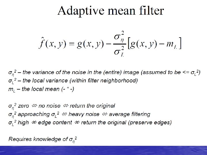
Adaptive, Local Noise Reduction Filter • Two parameters are considered: – Mean: measure of average gray level. – Variance: measure of average contrast. • Four measurements: (1) noisy image at (x, y ): g(x, y ) (2) The variance of noise 2 (3) The local mean m. L in Sxy (4) The local variance 2 L

Adaptive, Local Noise Reduction Filter Given the corrupted image g(x, y), find f(x, y). Conditions: (a) 2 is zero (Zero-noise case) – Simply return the value of g(x, y). (b) If 2 L is higher than 2 – Could be edge and should be preserved. – Return value close to g(x, y). (c) If 2 L = 2 – when the local area has similar properties with the overall image. – Return arithmetic mean value of the pixels in Sxy. General expression:

Adaptive, Local Noise Reduction Filter

Introduction Removes Impulse noise and Reduces Distortion along the boundaries Window size is variable to improve efficiency Removes Salt and Pepper noise Smoothens non-impulsive noise

Implementation Three cases were implemented: With Salt and Pepper noise alone With non impulsive noise alone With both included Variations in the window size were introduced Variations in the noise power were introduced

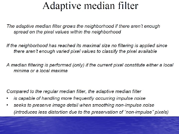
Adaptive Median Filter • Adaptive median filter can handle impulse • • noise with larger probability (Pa and Pb are large). This approach changes window size during operation (according to certain criteria). First, define the following notations: zmin=minimum gray-level value in Sxy zmax=maximum gray-level value in Sxy zmed=median gray-level value in Sxy zxy= gray-level at (x, y) Smax=maximum allowed size of Sxy

Adaptive Median Filter • The adaptive median filter algorithm works • in two levels: A and B Level A: A 1=zmed-zmin A 2=zmed-zmax If A 1>0 and A 2<0 goto level B else increase the window size If window size Smax repeat level A else output zxy Level B: B 1=zxy-zmin B 2=zxy-zmax If B 1>0 AND B 2<0, output zxy Else output zmed.

Example 5. 5

Salt and pepper noise Salt and Pepper Standard Median output Adaptive median Output

With Non-impulsive noise Gaussian Noise Standard Median output Adaptive Median Output

With both types of noise Gaussian and impulsive Noise Standard Median output Adaptive Median output

Conclusions • The adaptive median filter successfully removes • • impulsive noise from images. It does a reasonably good job of smoothening images that contain non -impulsive noise. When both types of noise are present, the algorithm is not as successful in removing impulsive noise and its performance deteriorates. Overall, the performance is as expected and the successful implementation of the adaptive median filter is presented.

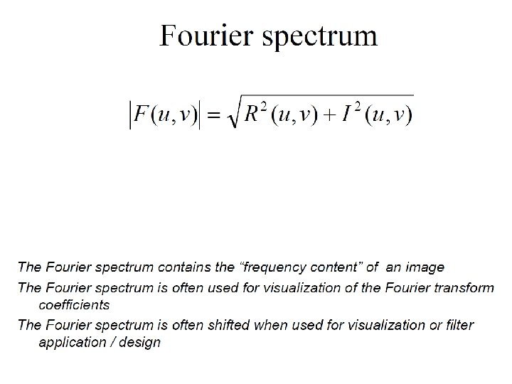
Image Enhancement in Frequency Domain

Image Enhancement Original image Enhanced image Enhancement: to process an image for more suitable output for a specific application. 40

Image Enhancement • Image enhancement techniques: Ø Spatial domain methods Ø Frequency domain methods • Spatial (time) domain techniques are techniques that operate directly on pixels. • Frequency domain techniques are based on modifying the Fourier transform of an image. 41

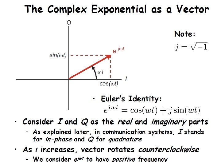
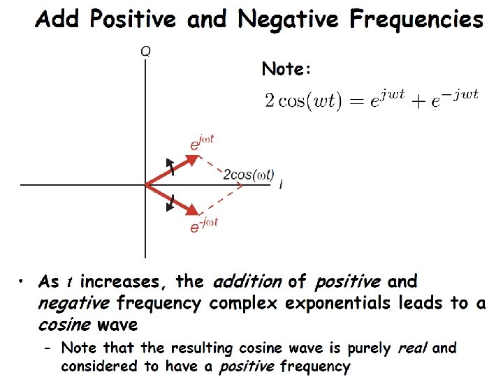
Fourier Transform: a review • Basic ideas: Ø A periodic function can be represented by the sum of sum sines/cosines functions of different frequencies, multiplied by a different coefficient. Ø Non-periodic functions can also be represented as the integral of sines/cosines integral multiplied by weighing function. 42

Joseph Fourier (1768 -1830) Fourier was obsessed with the physics of heat and developed the Fourier transform theory to model heatflow problems. 43

4. 2. 3 Filtering in the Frequency Domain • What is the “frequency” of an image? – Since frequency is directly related rate of change, it is not difficult intuitively to associate frequencies with pattern of intensity variations in an image. • The low frequencies correspond to the slowly varying components of an image. • The higher frequencies begin to correspond to faster and faster gray level changes in the image. – such as edges. – F(0, 0): the average gray level of an image.

Fourier transform basis functions Approximating a square wave as the sum of sine waves. 45

Any function can be written as the sum of an even and an odd function E(-x) = E(x) O(-x) = -O(x) 46

Fourier Cosine Series Because cos(mt) is an even function, we can write an even function, f(t), as: where series Fm is computed as Here we suppose f(t) is over the interval (–π, π). 47

Fourier Sine Series Because sin(mt) is an odd function, we can write any odd function, f(t), as: where the series F’m is computed as 48

Fourier Series So if f(t) is a general function, neither even nor odd, it can be written: Even component Odd component where the Fourier series is 49

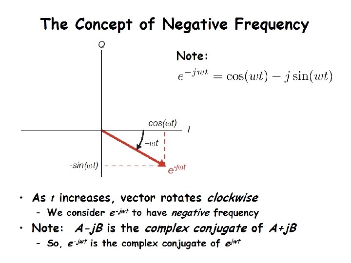
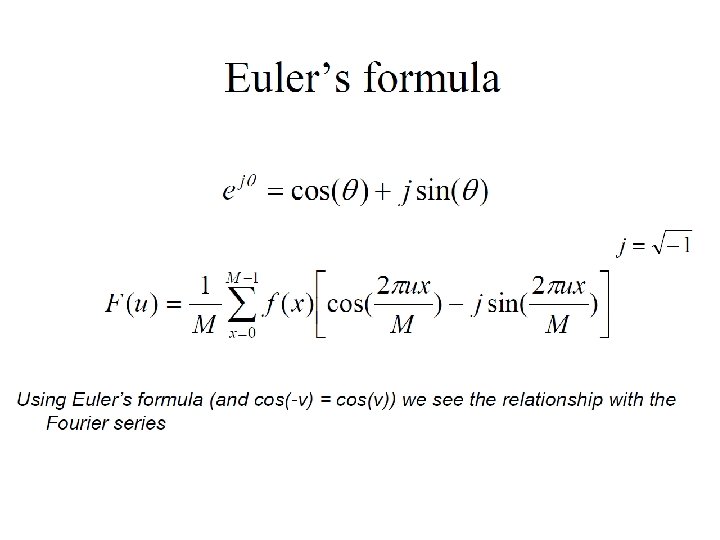
The Fourier Transform Let F(m) incorporates both cosine and sine series coefficients, with the sine series distinguished by making it the imaginary component: Let’s now allow f(t) range from – to , we rewrite: F(u) is called the Fourier Transform of f(t). We say that f(t) lives in the “time domain, ” and F(u) lives in the “frequency domain. ” u is called the frequency variable. 50

The Fourier Transform u· x 1/M 51

d a time domain frequency domain d = a + b + c b time domain frequency domain c time domain frequency domain 52

The Inverse Fourier Transform We go from f(t) to F(u) by Fourier Transform Given F(u), f(t) can be obtained by the inverse Fourier transform Inverse Fourier Transform 53

Discrete Fourier Transform (DFT) • A continuous function f(x) is discretized as: 54

Discrete Fourier Transform (DFT) Let x denote the discrete values (x=0, 1, 2, …, M-1), i. e. then 55

Discrete Fourier Transform (DFT) • The discrete Fourier transform pair that applies to sampled functions is given by: u=0, 1, 2, …, M-1 and x=0, 1, 2, …, M-1 56

2 -D Discrete Fourier Transform • In 2 -D case, the DFT pair is: u=0, 1, 2, …, M-1 and v=0, 1, 2, …, N-1 and: x=0, 1, 2, …, M-1 and y=0, 1, 2, …, N-1 57

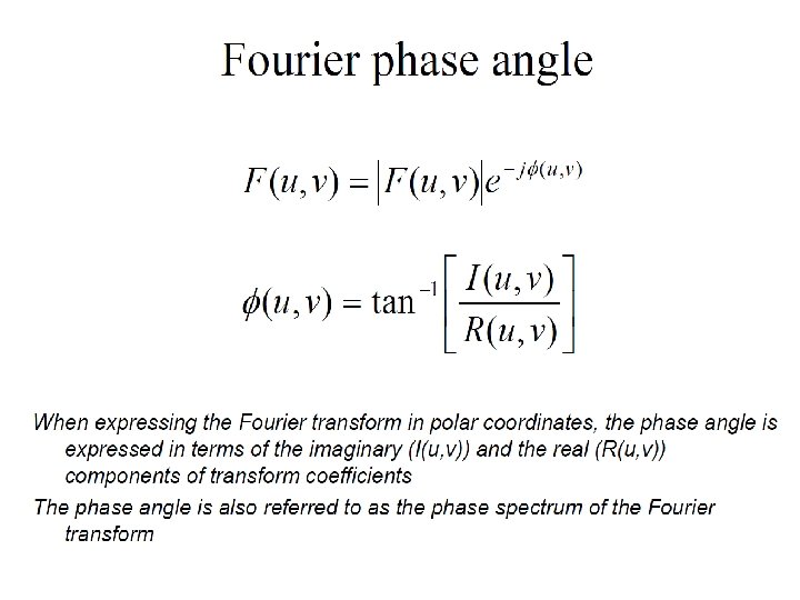
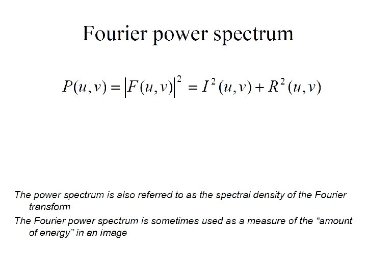
Polar Coordinate Representation of FT • The Fourier transform of a real function is generally complex and we use polar coordinates: Polar coordinate Magnitude: Phase: 63

Fourier Transform: shift • It is common to multiply input image by (-1)x+y prior to computing the FT. This shift the center of the FT to (M/2, N/2). Shift 64

Symmetry of FT • For real image f(x, y), FT is conjugate symmetric: • The magnitude of FT is symmetric: 65

FT IFT 66

IFT 67

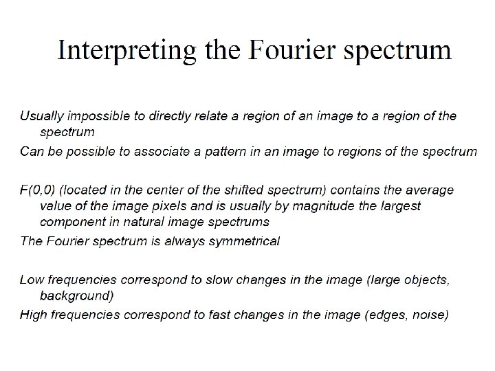
The central part of FT, i. e. the low frequency components are responsible for the general gray-level appearance of an image. The high frequency components of FT are responsible for the detail information of an image. 68

69

70

71

72

73

74

75

Image Frequency Domain (log magnitude) v Detail u General appearance 76

Examples of 2 DFT a a b b c c Image Fourier transform 77

5% 10 % 20 % 50 % 78

The End