Med PhysBME 574 Presentation Techniques for Tracking Fluorescent

Med Phys/BME 574 Presentation Techniques for Tracking Fluorescent Probes in the Optical Microscopy of Biological Molecules Minrui Yu Eric Stava Adam Uselmann 05/02/2008

Outline • Background of fluorescent imaging (Minrui) • Tracking algorithms (Eric) • Monte Carlo simulations and results (Adam)

Introduction • What is fluorescence imaging? – Imaging using the phenomena of fluorescence and instead of, or in addition to, reflection and absorption. – Fluorescence: absorption of photon emission of photon with longer wavelength + molecular vibration

Physics of fluorescence imaging Excitation Vibrational relax Emission

Vibrational energy levels and excitation and fluorescent spectra

• Why use fluorescence imaging? – Sensitivity: approach that of radioisotopes – Multicolor detection: target specific fluorescent labels for differentiation – Stability: long shelf-life up to 6 months – Low hazard: handle, storage, disposal – Availability and cost

Application examples St. Patrick’s Day Chicago River Fluorescence Microscopy

Biophotonic Imaging/Fluorescence Microscopy Veiseh et al, 2007 Olympus demo

• Particle tracking – Study intranuclear trajectories of single protein molecules, Kues et al, 2001 – video

Excitation sources • Ultraviolet (UV) light: wide spectrum • Laser: Ar laser: 457 nm, 488 nm, 514 nm Nd: YAG laser: 532 nm He/Ne laser: 633 nm • Light emitting diode (LED): >635 nm

Fluorescent Materials Fluorophore Protein Quantum dot

Molecule detection and tracking

Molecule detection and tracking • Particle localization accuracy: distance from the found object center, in which the true object center is located with a probability of 0. 68. • Sub-wavelength accuracy: 10 nm in x-, y-, z-direction • Signal to noise ratio (SNR)

Three types of images were acquired: • “dark current images” (camera shutter closed) • images of the specimen chamber containing only buffer • and images of intact and digitonin-permeabilized cells From these the mean fluorescence and its standard deviation (SD) were derived.

Tracking Algorithms • Used to track particles with subwavelength size and displacement • Two basic types – Estimate the absolute position of particles • Centroid (COM) algorithm • Gaussian fits algorithm – Estimate the change in position of particles • Cross-correlation • Sum-absolute Difference Cheezem, et. al. , Biophys J, 81 (2001), p. 2378 -2388

Gaussian Fits • The most common method for sub-wavelength particle tracking • Most sub-wavelength particles can be approximated by a point source of light • The peak of the PSF is well approximated by a Gaussian r = distance from origin NA = Numerical Aperture J 1 = Bessel Function Lambda = wavelength of light

Gaussian Fit Algorithm • Fit a 2 D Gaussian using a simplex algorithm with a least -squares estimator • Tracking is done by subtracting values of xo, yo from subsequent images xo , yo = center of the curve A, B = constants

Centroid (COM) Algorithm • Cx is calculated for one image and subtracted by the subsequent image • Especially susceptible to changes in particle shape or orientation • Assumes the object has higher intensity than background xi = Coordinate of pixel on x-axis I = Intensity at that pixel

Centroid - Thresholding • For centroid tracking, one must exclude as much image background as possible • Thresholding is typically used – Simple Thresholding: Values below threshold set to zero; those above unaltered – Binary Thresholding: Values below threshold set to zero; those above set to one • This helps to reduce a bias toward the center of an image

Correlation • Most computationally intensive of the techniques • Compares an image (I) to a kernel (K) of a successive image • K is shifted in one pixel increments, and a correlation value is calculated at each increment • At the shift where K and I are most similar, one finds a maximum in the correlation matrix X x, y = distance the kernal has moved over the original image

Normalized Correlation • Correlation tends to match the brightest regions of two images rather than the best topographical fit • Normalized Correlation: Each value in the correlation matrix is divided by the root mean square (RMS) of the original image intensities MK = RMS value of the kernel MIx, y = RMS value of the overlapping portion of the image

Normalized Covariance • Used when the image and kernel have a relative offset in intensity • Here, the mean of kernel K is subtracted from each cell in K, and the mean in I in the overlapping region is subtracted from each cell in I

Sum-absolute Difference • SAD method determines the translation of I relative to K that minimizes the sum of absolute differences between the overlapping pixels • Although this algorithm has never been used for tracking fluorescent particles, it is a standard algorithm for tracking the motion of features in medical imaging

Interpolation • In centroid and Gaussian fits, the position is calculated as an average over a set of coordinates, so the distance calculated inherently has sub-pixel resolution • SAD and correlation compare subsequent images, and so only offer whole-pixel estimates—interpolation is needed. • The data in the SAD or correlation matrices form quasi-paraboloid meshes.

Paraboloid Interpolation • x and y represent distances moved, z represents SAD or Correlation value • The peak of the correlation value (trough of SAD value) is set to z(x 0, y 0) = a. • This and the four immediately surrounding points are used to calculate the paraboloid coefficients • x and y are solved directly from the coefficients

Other Interpolation Methods • Cosine Interpolation Delta = peak of correlation function Omega = angular frequency of cosinusoid Theta = phase of cosinusoid • Gaussian Fit to Peak of Correlation Function

Image Model • Start with a high-resolution matrix (9 nm pixel size) • Insert an object (a “white” level of 10000 inside object, a “black” level of 0 everywhere else) • Convolve with the PSF to simulate the microscope objective r = distance from origin NA = Numerical Aperture J 1 = Bessel Function Lambda = wavelength of light

CCD Image Construction • Integrate over regions of matrix to form CCD pixel (1/11 resolution of high-resolution matrix) • Less than single CCD pixel displacements can be simulated • For 100 x magnification, we get 100 nm/pixel

Noise Model • Intensifiers in CCD cameras generate shot noise • Each CCD pixel observes N photoelectrons • N = 10 for black image; N = 15 -1000 for white image • Shot noise simulated by picking a random value from a Poisson distribution of mean N

Fitting Algorithm Comparison • Quantified by: • Bias error (accuracy) • Standard deviation (precision)

Fitting Algorithm Comparison

Fitting Algorithm Comparison

Summary • When the object is small (d < λ), Gaussian fit excels • When the object is large (d > λ), correlation method performed best • Below SNR = 4, everything fails – Bias exceeds one pixel in best case – SNR = 6 to 8 required for other methods

Nanometer localization of fluorescent probes • Gaussian fit algorithm – Series of Monte Carlo generated test images – Actual measured images • 30 nm diameter fluorescent beads • 130 nm pixel size

Monte Carlo – Probe Localization • Used to create test images – Random position chosen (Stochastic) – 2 D Gaussian intensity distribution integrated over each pixel (Deterministic) – Integrated intensity average replaced by Poisson distributed random number with same average (Stochastic) • Photon counting noise – Gaussian added with σ = b to simulate background noise (Stochastic) • Gaussian fit applied • Precision of localization determined based on number of detected photons

Monte Carlo – Probe Localization Ctd. • Optimal pixel size/spot size ratio Solid = Theoretical loc. , Dashed = Solid + 30% , Circles = MC generated test images

Probe Localization Results • Gaussian mask tracking Dashed = Monte Carlo, Solid = Theoretical, Circles = Measured

MC Probe Localization Summary • MC methods used to generate test images – Used to check accuracy and precision of algorithm – Comparison to measured results • Used to determine optimal imaging parameters – Pixel size/spot size

Protein Visualization • Molecular diffusion • Nucleus modeled as ellipsoid – Axes of 15, 20, and 6 μm • Assumes Brownian motion – Diffusion const. of 2. 5 μm 2/s – Various time steps • Observation slice 0. 8 μm thick in x-y plane

Protein trajectories

Protein Trajectories

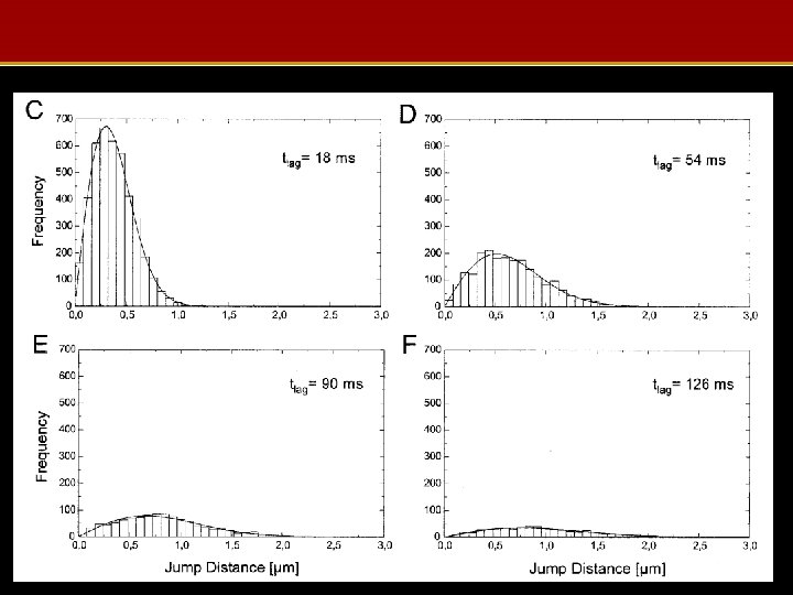
Measured Jump Distances

MC Protein Visualization Summary • MC used to model protein trajectories in nucleus • Varying diffusion parameters gives jump distance/time curves – Fitted to measured jump distances to give distribution of protein mobilities

Conclusion • Microscopy may be used to image individual molecules within a cell – In vitro, non-clinical • Algorithms may be applied to images to achieve sub-pixel size localization – Nanometer scale • Monte Carlo may augment experiments – Verify experimental results – Determine effective imaging parameters