Measuring Poverty Inequality Measures n n n n

Measuring Poverty: Inequality Measures n n n n Charting Inequality Share of Expenditure of Poor Dispersion Ratios Lorenz Curve Gini Coefficient Theil Index Comparisons Decomposition 1

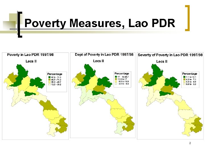
Poverty Measures, Lao PDR 2

Income Distribution n Types of analysis ¡ ¡ n Functional distribution— ¡ n Functional distribution Size distribution income accrued to factors of production such as land, labor, capital and entrepreneurship Size distribution— ¡ income received by different households or individuals 3

What is Inequality? n Dispersion or variation of the distribution of income/consumption or other welfare indicator ¡ ¡ Equality– everyone has the same income Inequality– certain groups of the population have higher incomes compared to other groups in the population 4

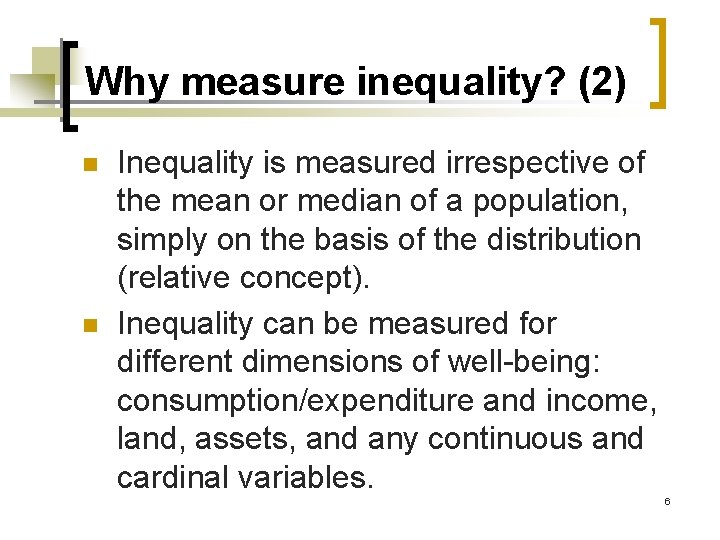
Why measure inequality? (1) n Indicator of well-being ¡ ¡ n “Position” of individual relative to rest of population “Position” of subgroup relative to other subgroups Different measures, different focus ¡ ¡ Poverty measures (HC, PGI, SPGI, etc) focus on the situation of individuals who are below the poverty line– the poor. Inequality is defined over the entire 5

Why measure inequality? (2) n n Inequality is measured irrespective of the mean or median of a population, simply on the basis of the distribution (relative concept). Inequality can be measured for different dimensions of well-being: consumption/expenditure and income, land, assets, and any continuous and cardinal variables. 6

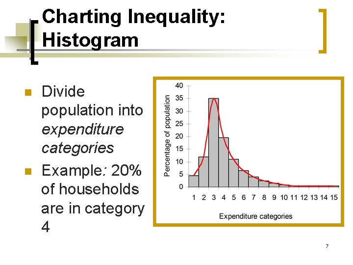
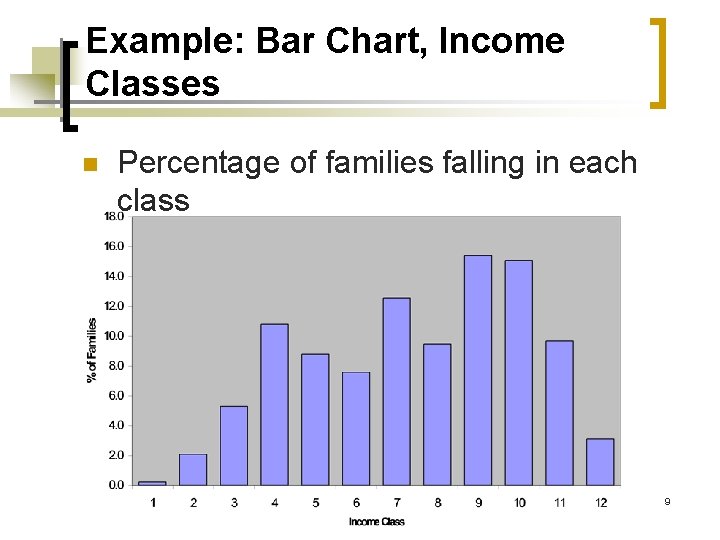
Charting Inequality: Histogram n n Divide population into expenditure categories Example: 20% of households are in category 4 7

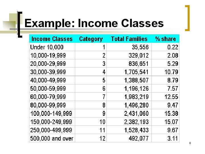
Example: Income Classes 8

Example: Bar Chart, Income Classes n Percentage of families falling in each class 9

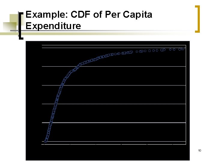
Example: CDF of Per Capita Expenditure 10

Distribution: Quintile and Deciles 11

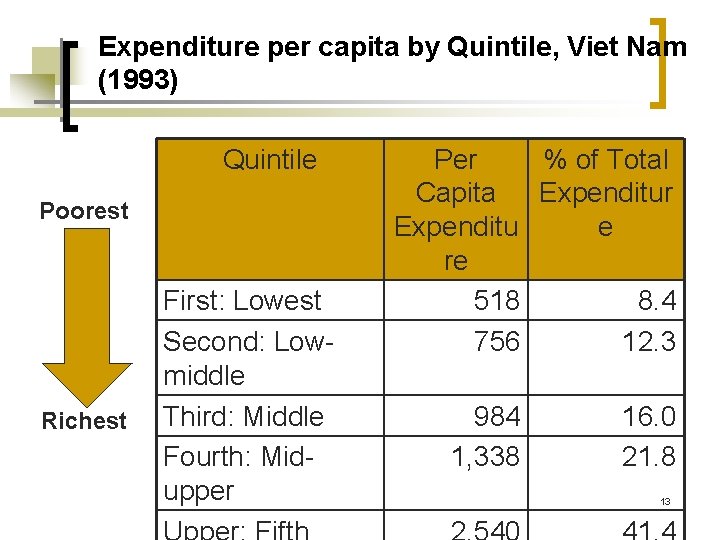
Expenditure/Income-iles n n Divide population into ‘groups’ ranked from ‘poorest’ to ‘richest’ based on expenditure (or income) Divide into 5 groups: income or expenditure quintiles ¡ ¡ n Lowest 20% or first quintile– “poorest” Highest 20% or fifth quintile– “richest” Divide into 10 groups: income or expenditure deciles 12

Expenditure per capita by Quintile, Viet Nam (1993) Quintile Poorest Richest First: Lowest Second: Lowmiddle Third: Middle Fourth: Midupper Per % of Total Capita Expenditur Expenditu e re 518 8. 4 756 12. 3 984 1, 338 16. 0 21. 8 13

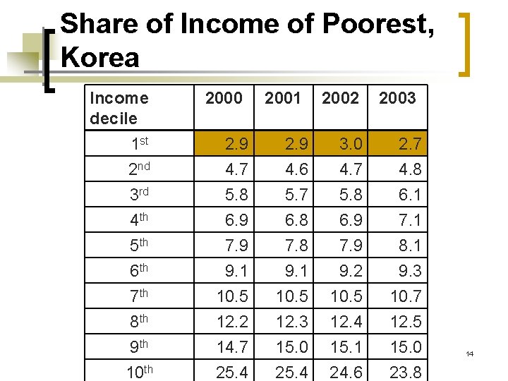
Share of Income of Poorest, Korea Income decile 1 st 2 nd 3 rd 4 th 5 th 6 th 7 th 8 th 9 th 10 th 2000 2. 9 4. 7 5. 8 6. 9 7. 9 9. 1 10. 5 12. 2 14. 7 25. 4 2001 2. 9 4. 6 5. 7 6. 8 7. 8 9. 1 10. 5 12. 3 15. 0 25. 4 2002 3. 0 4. 7 5. 8 6. 9 7. 9 9. 2 10. 5 12. 4 15. 1 24. 6 2003 2. 7 4. 8 6. 1 7. 1 8. 1 9. 3 10. 7 12. 5 15. 0 23. 8 14

Inequality Measures Based on -iles n n Share of income/consumption of lowest –ile Dispersion ratios 15

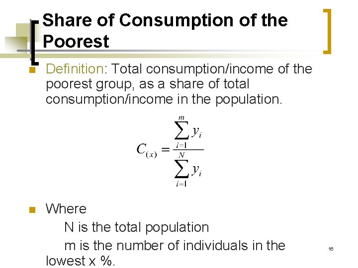
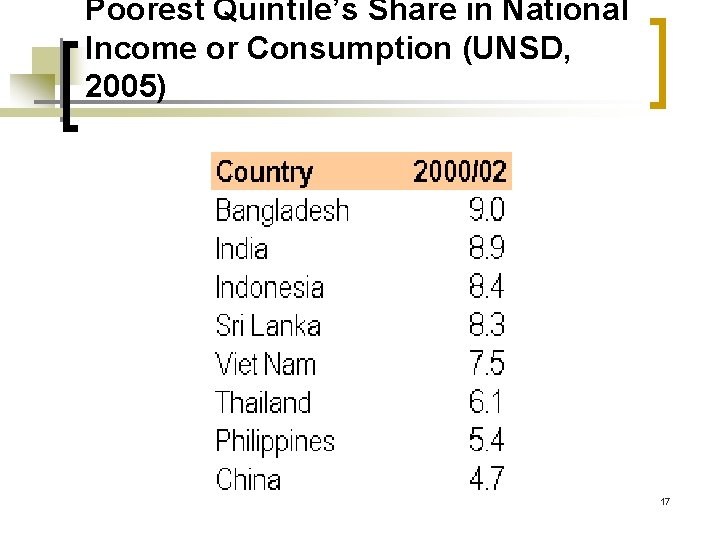
Share of Consumption of the Poorest n Definition: Total consumption/income of the poorest group, as a share of total consumption/income in the population. n Where N is the total population m is the number of individuals in the lowest x %. 16

Poorest Quintile’s Share in National Income or Consumption (UNSD, 2005) 17

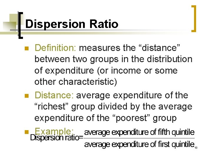
Dispersion Ratio n n n Definition: measures the “distance” between two groups in the distribution of expenditure (or income or some other characteristic) Distance: average expenditure of the “richest” group divided by the average expenditure of the “poorest” group Example: 18

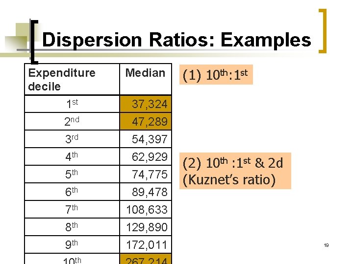
Dispersion Ratios: Examples Expenditure decile 1 st 2 nd 3 rd 4 th 5 th 6 th 7 th 8 th 9 th th Median (1) 10 th: 1 st 37, 324 47, 289 54, 397 62, 929 74, 775 89, 478 108, 633 129, 890 172, 011 (2) 10 th : 1 st & 2 d (Kuznet’s ratio) 19

Lorenz Curve and Gini Ratio 20

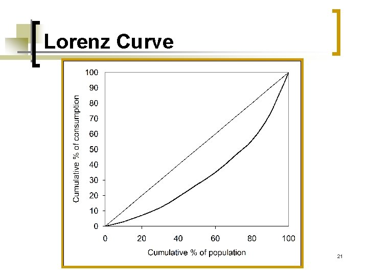
Lorenz Curve 21

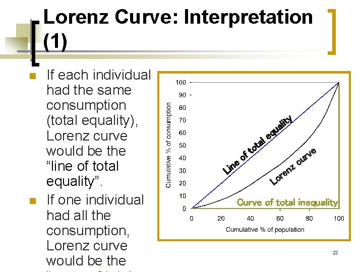
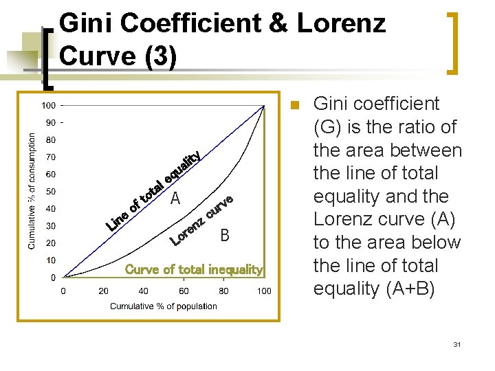
Lorenz Curve: Interpretation (1) n n If each individual had the same consumption (total equality), Lorenz curve would be the “line of total equality”. If one individual had all the consumption, Lorenz curve would be the ty i l a u a e n i L ot t f q e l ve r u o c z n e r o L Curve of total inequality 22

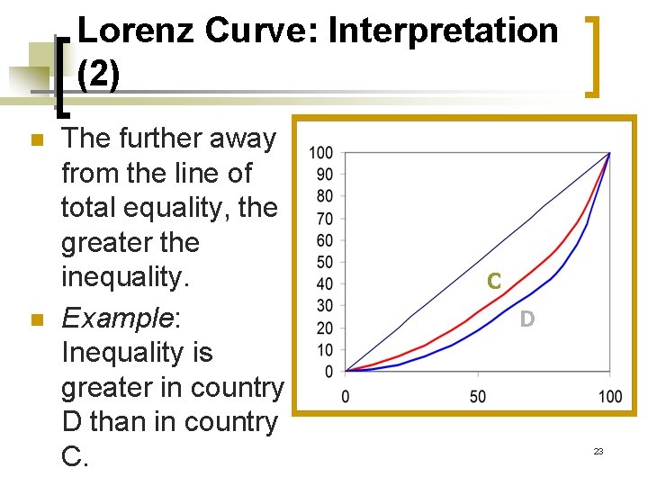
Lorenz Curve: Interpretation (2) n n The further away from the line of total equality, the greater the inequality. Example: Inequality is greater in country D than in country C. C D 23

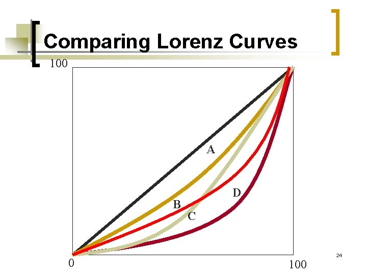
Comparing Lorenz Curves 100 A B 0 D C 100 24

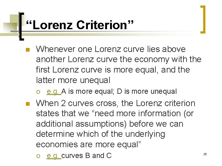
“Lorenz Criterion” n Whenever one Lorenz curve lies above another Lorenz curve the economy with the first Lorenz curve is more equal, and the latter more unequal ¡ n e. g. A is more equal; D is more unequal When 2 curves cross, the Lorenz criterion states that we “need more information (or additional assumptions) before we can determine which of the underlying economies are more equal” ¡ e. g. curves B and C 25

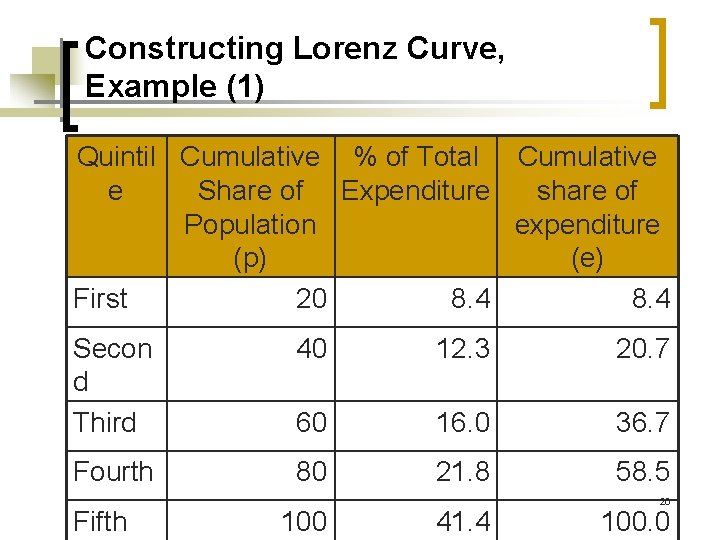
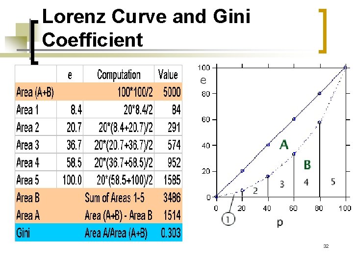
Constructing Lorenz Curve, Example (1) Quintil Cumulative % of Total Cumulative e Share of Expenditure share of Population expenditure (p) (e) First 20 8. 4 Secon d Third 40 12. 3 20. 7 60 16. 0 36. 7 Fourth 80 21. 8 58. 5 Fifth 100 41. 4 26 100. 0

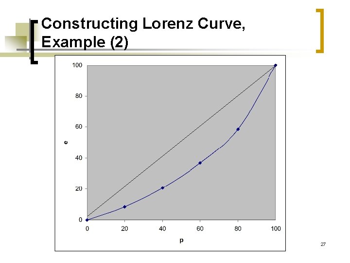
Constructing Lorenz Curve, Example (2) 27

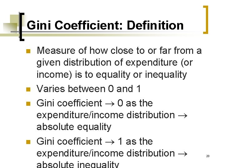
Gini Coefficient: Definition n n Measure of how close to or far from a given distribution of expenditure (or income) is to equality or inequality Varies between 0 and 1 Gini coefficient 0 as the expenditure/income distribution absolute equality Gini coefficient 1 as the expenditure/income distribution 28

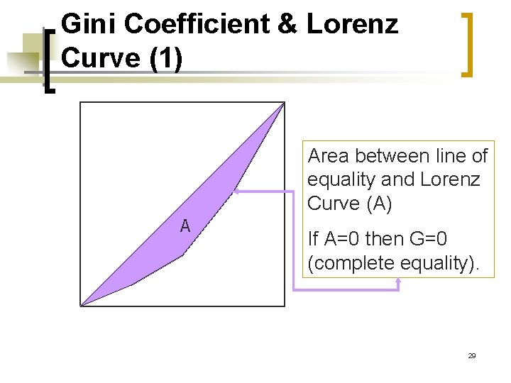
Gini Coefficient & Lorenz Curve (1) Area between line of equality and Lorenz Curve (A) A If A=0 then G=0 (complete equality). 29

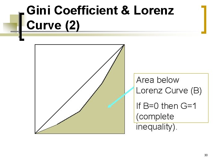
Gini Coefficient & Lorenz Curve (2) Area below Lorenz Curve (B) If B=0 then G=1 (complete inequality). 30

Gini Coefficient & Lorenz Curve (3) n ty i l a l e n i L of t a ot u q e A Lo nz e r ve r cu B Curve of total inequality Gini coefficient (G) is the ratio of the area between the line of total equality and the Lorenz curve (A) to the area below the line of total equality (A+B) 31

Lorenz Curve and Gini Coefficient e 32

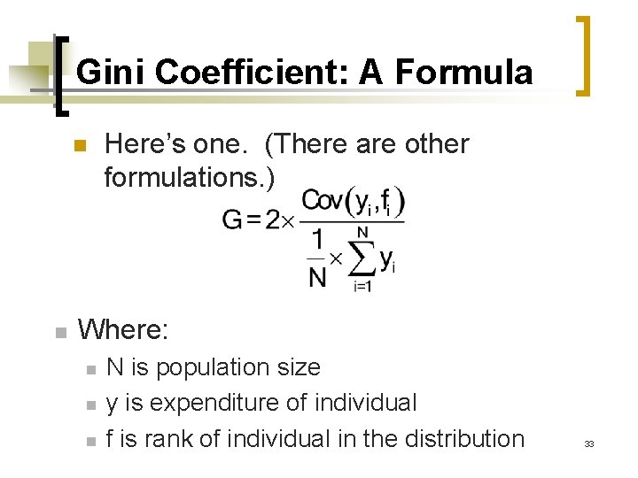
Gini Coefficient: A Formula n n Here’s one. (There are other formulations. ) Where: n n n N is population size y is expenditure of individual f is rank of individual in the distribution 33

Gini Coefficient: +’s and –’s n n n (+) Easy to understand, in light of the Lorenz curve. (-) Not decomposable: the total Gini of the total population is not equal to the sum of the Ginis for its subgroups. (-) Sensitive to changes in the distribution, irrespective of whether they take place at the top, the middle or the bottom of the distribution (any transfer of income between two individuals has an impact, irrespective of whether it occurs among the rich or among the poor). 34

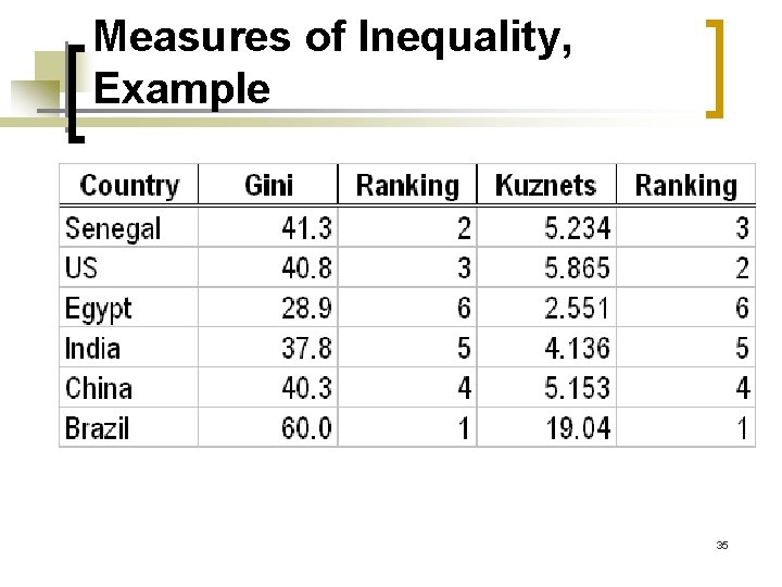
Measures of Inequality, Example 35

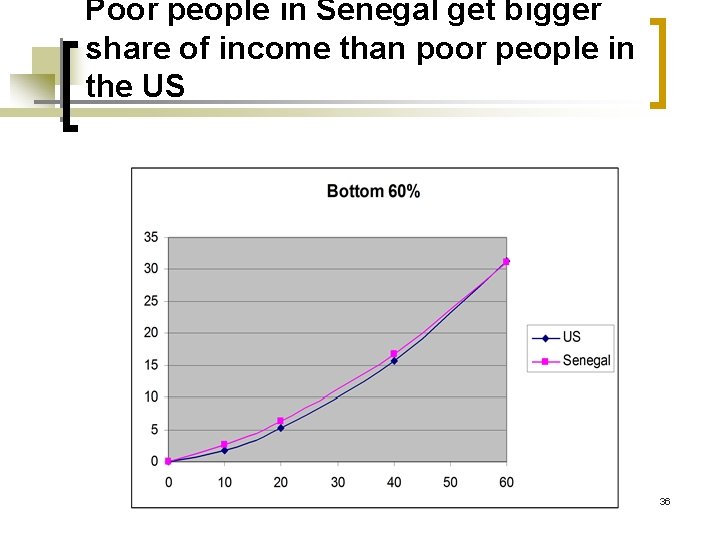
Poor people in Senegal get bigger share of income than poor people in the US 36

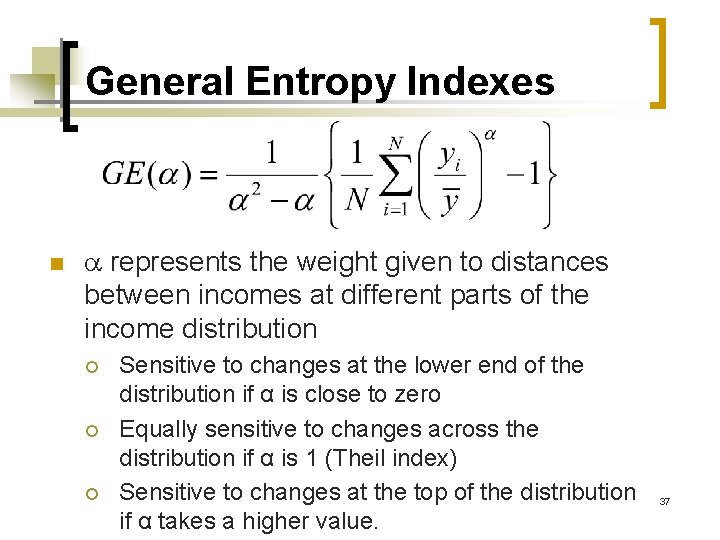
General Entropy Indexes n represents the weight given to distances between incomes at different parts of the income distribution ¡ ¡ ¡ Sensitive to changes at the lower end of the distribution if α is close to zero Equally sensitive to changes across the distribution if α is 1 (Theil index) Sensitive to changes at the top of the distribution if α takes a higher value. 37

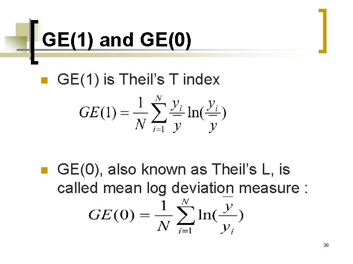
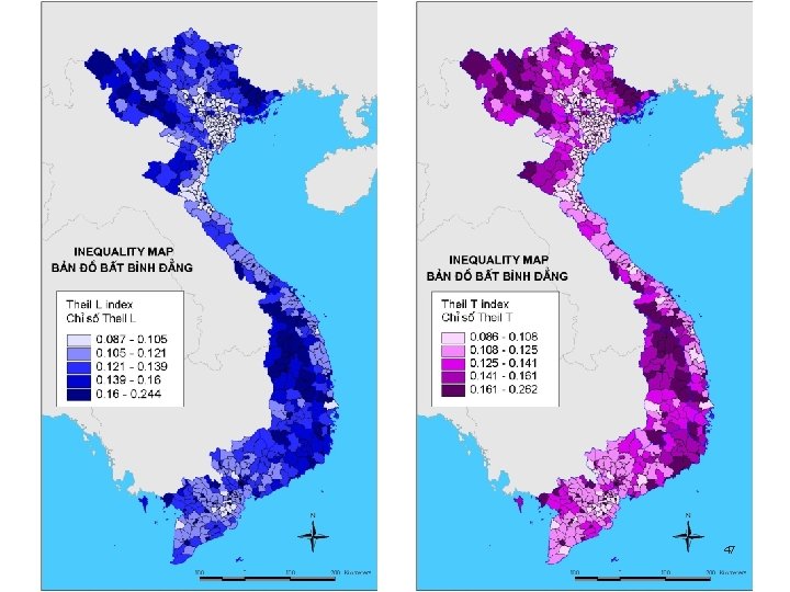
GE(1) and GE(0) n GE(1) is Theil’s T index n GE(0), also known as Theil’s L, is called mean log deviation measure : 38

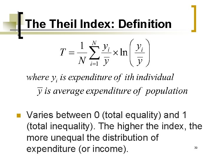
The Theil Index: Definition n Varies between 0 (total equality) and 1 (total inequality). The higher the index, the more unequal the distribution of expenditure (or income). 39

Theil Index: +’s and –’s) n n (+) Gives more weight to those at the bottom of the income distribution. (+) Can be decomposed into “sub-groups”: the population Theil is the weighted average of the index for each sub-group where the weights are population shares of each subgroup (-) Difficult to interpret (-) Sensitive to changes in the distribution, irrespective of whether they take place at the top, the middle or the bottom of the distribution (any transfer of income between two individuals has an impact, irrespective of whether it occurs among the rich or among 40

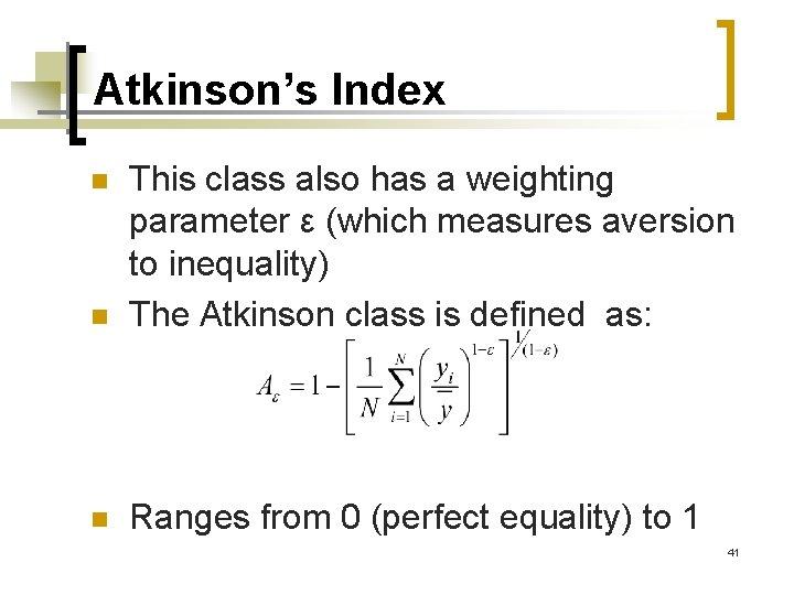
Atkinson’s Index n This class also has a weighting parameter ε (which measures aversion to inequality) The Atkinson class is defined as: n Ranges from 0 (perfect equality) to 1 n 41

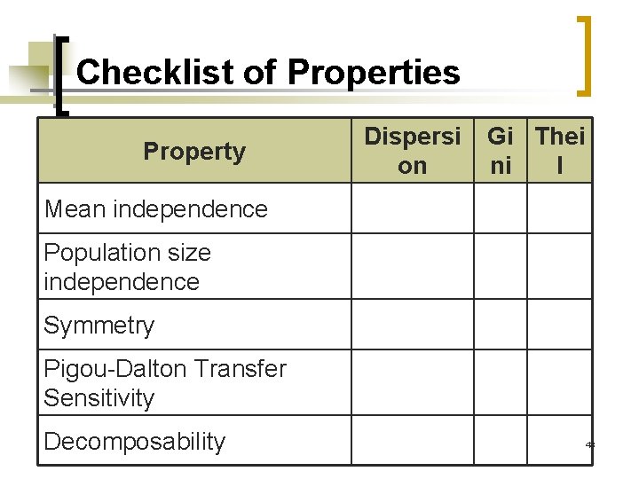
Criteria for ‘Goodness’ of Measures n n n Mean independence– If all incomes are doubled, measure does not change. Population size independence– If population size changes, measure does not change. Symmetry– If two individuals swap incomes, the measure does not change. Pigou-Dalton transfer sensitivity– Transfer of income from rich to poor reduces value of measure. Decomposability– It should be possible to break down total inequality by population groups, income source, expenditure type, or other dimensions. 42

Checklist of Properties Property Dispersi on Gi Thei ni l Mean independence Population size independence Symmetry Pigou-Dalton Transfer Sensitivity Decomposability 43

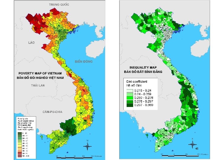
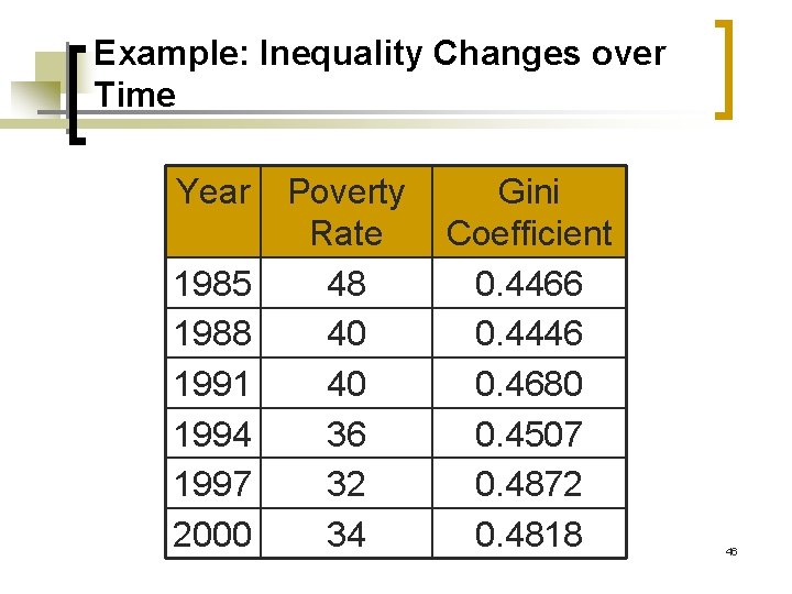
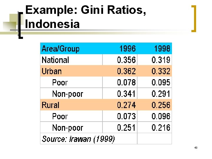
Inequality Comparisons n n Extent and nature of inequality among certain groups of households. This informs on the homogeneity of the various groups, an important element to take into account when designing interventions. Nature of changes in inequality over time. One could focus on changes for different groups of the population to show whether inequality changes have been similar for all or have taken place, say, in a particular sector of the economy. 44

45

Example: Inequality Changes over Time Year 1985 1988 1991 1994 1997 2000 Poverty Rate 48 40 40 36 32 34 Gini Coefficient 0. 4466 0. 4446 0. 4680 0. 4507 0. 4872 0. 4818 46

47

Example: Gini Ratios, Indonesia 48

Decomposition of Inequality 49

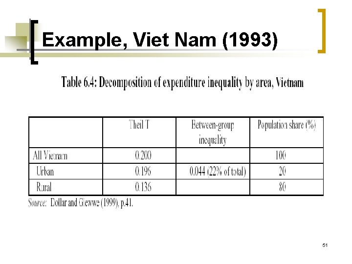
At One Point in Time (1) n n Inequality decompositions are typically used to estimate the share of total inequality in a country which results from different groups, from different regions or from different sources of income. Inequality can be decomposed into “between -group” components and “within-group” components. The first reflects inequality between people in different sub-groups (different educational, occupational, gender, geographic characteristics). The second reflects inequality among those people within the same sub-group. 50

Example, Viet Nam (1993) 51

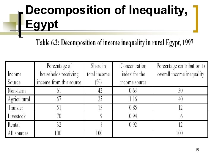
Decomposition of Inequality, Egypt 52

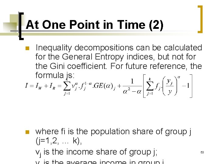
At One Point in Time (2) n Inequality decompositions can be calculated for the General Entropy indices, but not for the Gini coefficient. For future reference, the formula is: n where fi is the population share of group j (j=1, 2, … k), vj is the income share of group j; 53

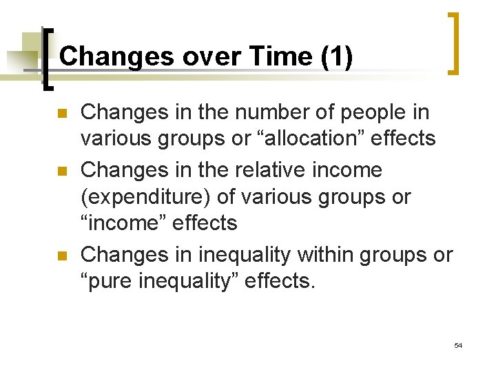
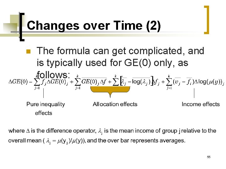
Changes over Time (1) n n n Changes in the number of people in various groups or “allocation” effects Changes in the relative income (expenditure) of various groups or “income” effects Changes in inequality within groups or “pure inequality” effects. 54

Changes over Time (2) n The formula can get complicated, and is typically used for GE(0) only, as follows: 55

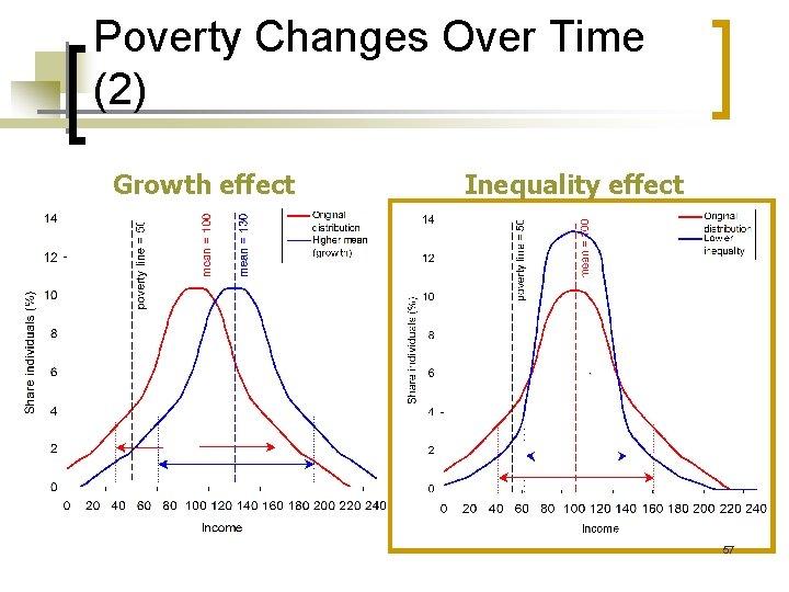
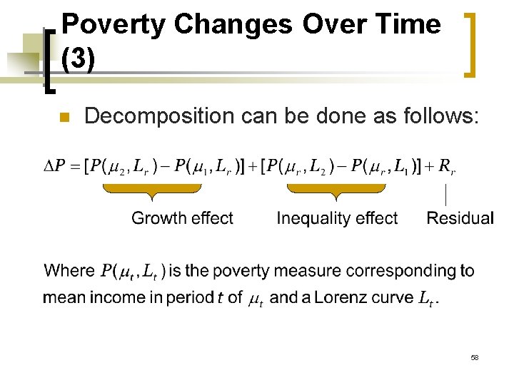
Poverty Changes over Time (1) n n Poverty is fully determined by the mean income or consumption of a population, and the inequality in income or consumption in the population. Changes in poverty can result from changes in mean income/consumption – growth – or from changes in inequality. 56

Poverty Changes Over Time (2) Growth effect Inequality effect 57

Poverty Changes Over Time (3) n Decomposition can be done as follows: 58

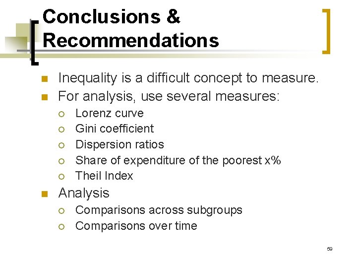
Conclusions & Recommendations n n Inequality is a difficult concept to measure. For analysis, use several measures: ¡ ¡ ¡ n Lorenz curve Gini coefficient Dispersion ratios Share of expenditure of the poorest x% Theil Index Analysis ¡ ¡ Comparisons across subgroups Comparisons over time 59