Measuring FX Exposure Transaction Exposure 1 FX Risk

Measuring FX Exposure Transaction Exposure 1

FX Risk Management FX Exposure: Review • At the firm level, currency risk is called exposure. • TE is simply to calculate: Value in DC of a specific transaction wit a certain date/maturity denominated in FC. • We can measure TE, and analyze the sensitivity of TE to changes in St. - Use a statistical distribution or a simulation. The less sensitive TE is to St, the lower the need to pay attention to ef, t. • MNCs have measures for NTE for: - a single transaction - all transactions (Netting, where co-movements of St‘s are incorporated

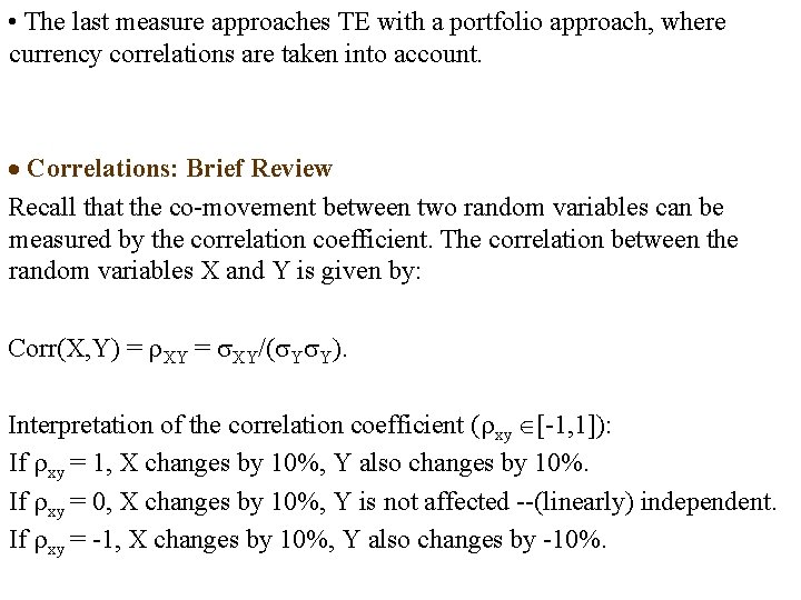
• The last measure approaches TE with a portfolio approach, where currency correlations are taken into account. Correlations: Brief Review Recall that the co-movement between two random variables can be measured by the correlation coefficient. The correlation between the random variables X and Y is given by: Corr(X, Y) = XY/( Y Y). Interpretation of the correlation coefficient ( xy [-1, 1]): If xy = 1, X changes by 10%, Y also changes by 10%. If xy = 0, X changes by 10%, Y is not affected --(linearly) independent. If xy = -1, X changes by 10%, Y also changes by -10%.

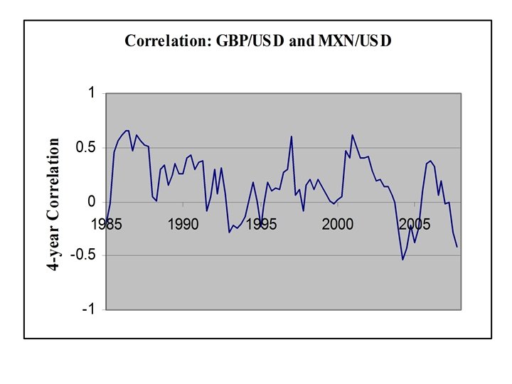
Currencies from developed countries tend to move together. . . But, not always!

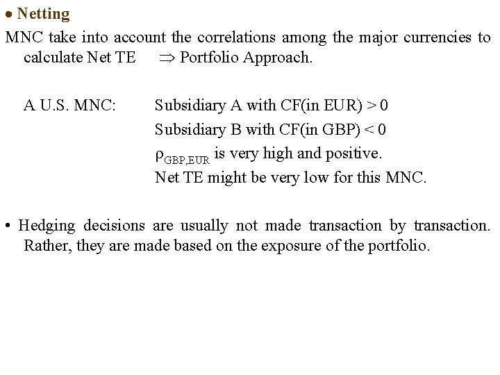
Netting MNC take into account the correlations among the major currencies to calculate Net TE Portfolio Approach. A U. S. MNC: Subsidiary A with CF(in EUR) > 0 Subsidiary B with CF(in GBP) < 0 GBP, EUR is very high and positive. Net TE might be very low for this MNC. • Hedging decisions are usually not made transaction by transaction. Rather, they are made based on the exposure of the portfolio.

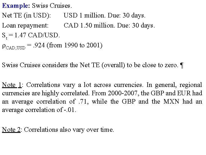
Example: Swiss Cruises. Net TE (in USD): USD 1 million. Due: 30 days. Loan repayment: CAD 1. 50 million. Due: 30 days. St = 1. 47 CAD/USD. CAD, USD =. 924 (from 1990 to 2001) Swiss Cruises considers the Net TE (overall) to be close to zero. ¶ Note 1: Correlations vary a lot across currencies. In general, regional currencies are highly correlated. From 2000 -2007, the GBP and EUR had an average correlation of . 71, while the GBP and the MXN had an average correlation of -. 01. Note 2: Correlations also vary over time.

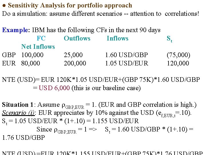
● Sensitivity Analysis for portfolio approach Do a simulation: assume different scenarios -- attention to correlations! Example: IBM has the following CFs in the next 90 days FC Outflows Inflows St Net Inflows GBP 100, 000 25, 000 1. 60 USD/GBP (75, 000) EUR 80, 000 200, 000 1. 05 USD/EUR 120, 000 NTE (USD)= EUR 120 K*1. 05 USD/EUR+(GBP 75 K)*1. 60 USD/GBP = USD 6, 000 (this is our baseline case) Situation 1: Assume GBP, EUR = 1. (EUR and GBP correlation is high. ) Scenario (i): EUR appreciates by 10% against the USD (ef, EUR, t=. 10). St = 1. 05 USD/EUR * (1+. 10) = 1. 155 USD/EUR Since GBP, EUR = 1 => St = 1. 60 USD/GBP * (1+. 10) = 1. 76 USD/GBP

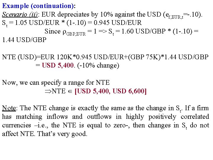
Example (continuation): Scenario (ii): EUR depreciates by 10% against the USD (ef, EUR, t=-. 10). St = 1. 05 USD/EUR * (1 -. 10) = 0. 945 USD/EUR Since GBP, EUR = 1 => St = 1. 60 USD/GBP * (1 -. 10) = 1. 44 USD/GBP NTE (USD)=EUR 120 K*0. 945 USD/EUR+(GBP 75 K)*1. 44 USD/GBP = USD 5, 400. (-10% change) Now, we can specify a range for NTE ∈ [USD 5, 400, USD 6, 600] Note: The NTE change is exactly the same as the change in St. If a firm has matching inflows and outflows in highly positively correlated currencies –i. e. , the NTE is equal to zero-, then changes in St do not affect NTE. That’s very good.

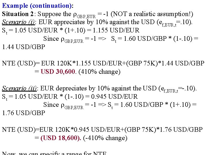
Example (continuation): Situation 2: Suppose the GBP, EUR = -1 (NOT a realistic assumption!) Scenario (i): EUR appreciates by 10% against the USD (ef, EUR, t=. 10). St = 1. 05 USD/EUR * (1+. 10) = 1. 155 USD/EUR Since GBP, EUR = -1 => St = 1. 60 USD/GBP * (1 -. 10) = 1. 44 USD/GBP NTE (USD)= EUR 120 K*1. 155 USD/EUR+(GBP 75 K)*1. 44 USD/GBP = USD 30, 600. (410% change) Scenario (ii): EUR depreciates by 10% against the USD (ef, EUR, t=-. 10). St = 1. 05 USD/EUR * (1 -. 10) = 0. 945 USD/EUR Since GBP, EUR = -1 => St = 1. 60 USD/GBP * (1+. 10) = 1. 76 USD/GBP NTE (USD)=EUR 120 K*0. 945 USD/EUR+(GBP 75 K)*1. 76 USD/GBP = (USD 18, 600). (-410% change)

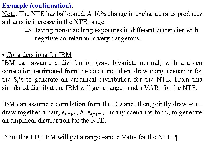
Example (continuation): Note: The NTE has ballooned. A 10% change in exchange rates produces a dramatic increase in the NTE range. Having non-matching exposures in different currencies with negative correlation is very dangerous. • Considerations for IBM can assume a distribution (say, bivariate normal) with a given correlation (estimated from the data) and, then, draw many scenarios for the St’s to generate an empirical distribution for the NTE. From this simulated distribution, IBM will get a range –and a VAR- for the NTE. IBM can assume a correlation from the ED and, then, jointly draw –i. e. , draw together a pair, ef, GBP, t & ef, EUR, t– many scenarios for St to generate an empirical distribution for the NTE. From this ED, IBM will get a range –and a Va. R- for the NTE. ¶