Measuring cause and effect of process variables Margret

Measuring cause and effect of process variables Margret Bauer, Nina F. Thornhill University College London John W. Cox Eastman Chemical Company APC Conference Vancouver, 9 -11 May 2005 1

Agenda Motivation Method Case Study Conclusion 2

Problem: Plant-wide disturbances in chemical plants act on many process variables TI 2 TC 1 TI 3 TI 6 DP 2 DP 1 TI 4 TI 7 TI 5 LI 2 LC 1 TI 1 The disturbances affect cost, quality and safety of a process. 3

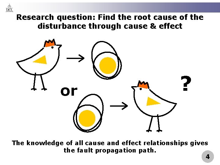
Research question: Find the root cause of the disturbance through cause & effect or ? The knowledge of all cause and effect relationships gives the fault propagation path. 4

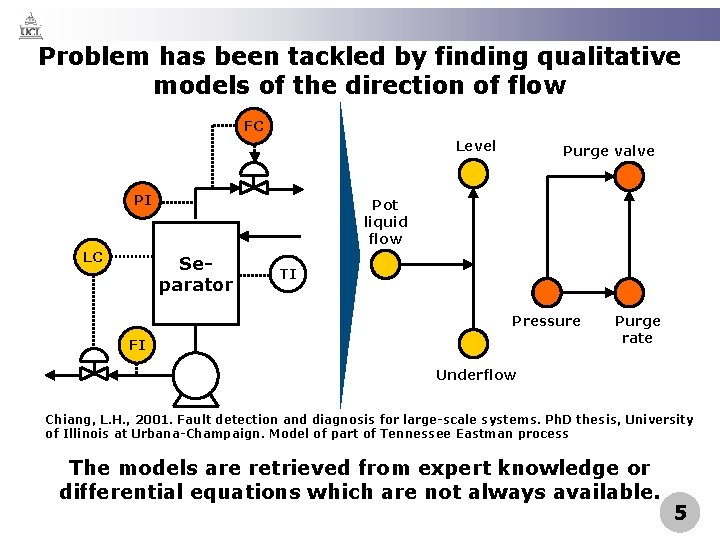
Problem has been tackled by finding qualitative models of the direction of flow FC Level PI LC Purge valve Pot liquid flow Separator TI Pressure FI Purge rate Underflow Chiang, L. H. , 2001. Fault detection and diagnosis for large-scale systems. Ph. D thesis, University of Illinois at Urbana-Champaign. Model of part of Tennessee Eastman process The models are retrieved from expert knowledge or differential equations which are not always available. 5

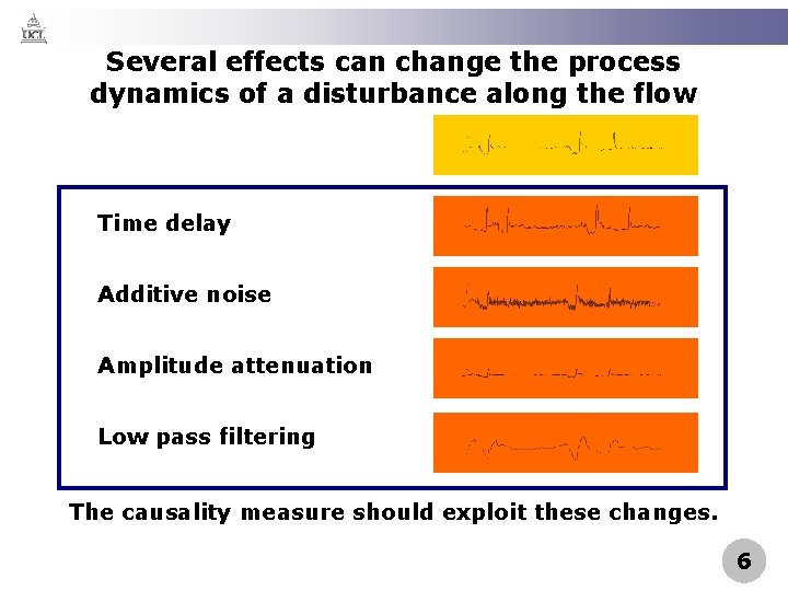
Several effects can change the process dynamics of a disturbance along the flow Time delay Additive noise Amplitude attenuation Low pass filtering The causality measure should exploit these changes. 6

Agenda Motivation Method Case Study Conclusion 7

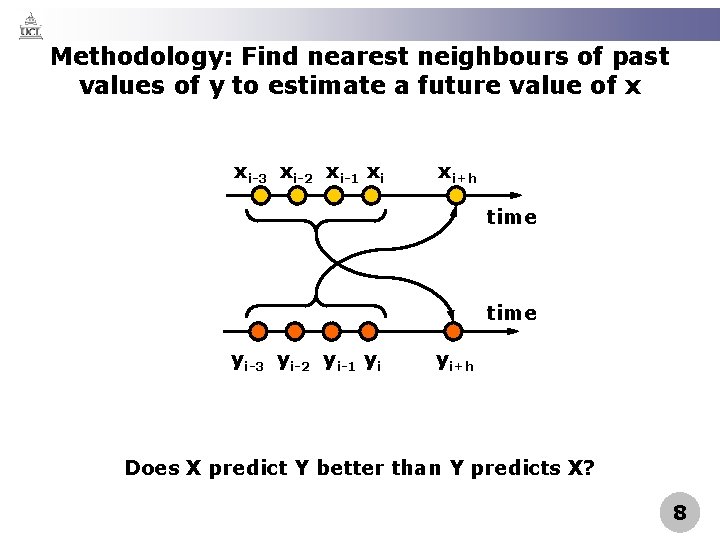
Methodology: Find nearest neighbours of past values of y to estimate a future value of x xi-3 xi-2 xi-1 xi xi+h time yi-3 yi-2 yi-1 yi yi+h Does X predict Y better than Y predicts X? 8

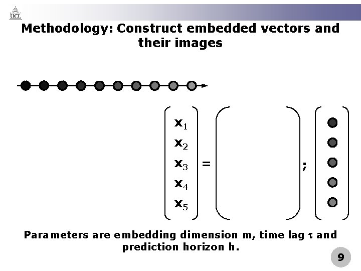
Methodology: Construct embedded vectors and their images x 1 x 2 x 3 = ; x 4 x 5 Parameters are embedding dimension m, time lag and prediction horizon h. 9

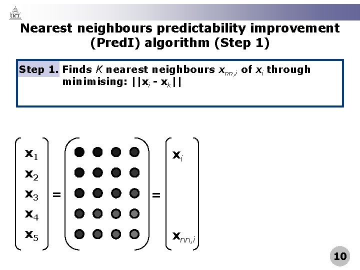
Nearest neighbours predictability improvement (Pred. I) algorithm (Step 1) Step 1. Finds K nearest neighbours xnn, i of xi through minimising: ||xi - xk|| x 1 xi x 2 x 3 = = x 4 x 5 xnn, i 10

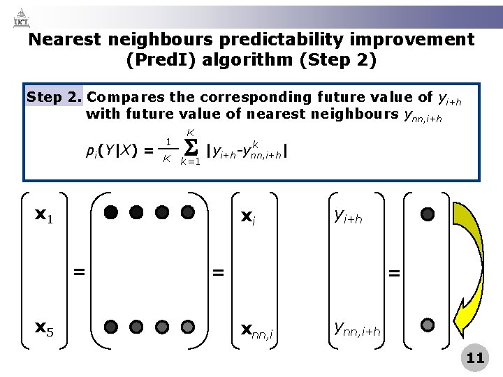
Nearest neighbours predictability improvement (Pred. I) algorithm (Step 2) Step 2. Compares the corresponding future value of yi+h with future value of nearest neighbours ynn, i+h pi(Y|X) = 1 K K k |yi+h-ynn, i+h | k=1 x 1 xi = x 5 yi+h = = xnn, i ynn, i+h 11

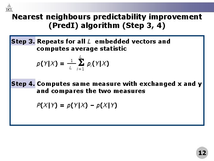
Nearest neighbours predictability improvement (Pred. I) algorithm (Step 3, 4) Step 3. Repeats for all L embedded vectors and computes average statistic p(Y|X) = 1 L L pi(Y|X) i=1 Step 4. Computes same measure with exchanged x and y and compares the two measures P(X|Y) = p(Y|X) – p(X|Y) 12

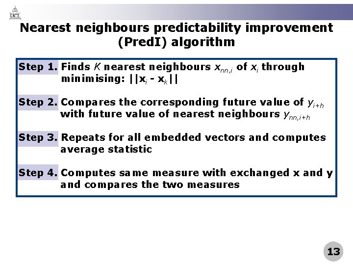
Nearest neighbours predictability improvement (Pred. I) algorithm Step 1. Finds K nearest neighbours xnn, i of xi through minimising: ||xi - xk|| Step 2. Compares the corresponding future value of yi+h with future value of nearest neighbours ynn, i+h Step 3. Repeats for all embedded vectors and computes average statistic Step 4. Computes same measure with exchanged x and y and compares the two measures 13

Agenda Motivation Method Case Study Conclusion 14

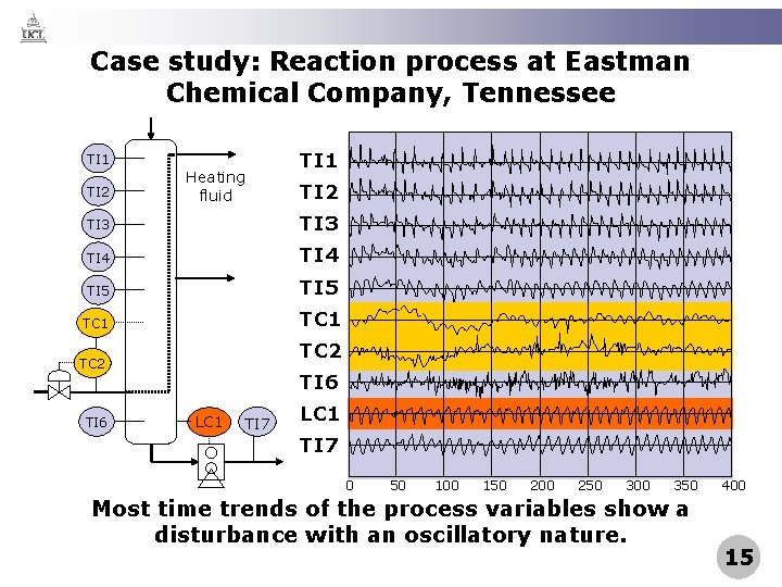
Case study: Reaction process at Eastman Chemical Company, Tennessee TI 1 TI 2 Heating fluid TI 1 TI 2 TI 3 TI 4 TI 5 TC 1 TC 2 TI 6 LC 1 TI 7 0 50 100 150 200 250 300 350 Most time trends of the process variables show a disturbance with an oscillatory nature. 400 15

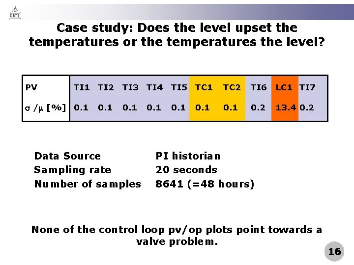
Case study: Does the level upset the temperatures or the temperatures the level? PV TI 1 TI 2 / [%] 0. 1 TI 3 TI 4 TI 5 TC 1 TC 2 TI 6 LC 1 TI 7 0. 1 0. 2 13. 4 0. 2 Data Source Sampling rate Number of samples 0. 1 PI historian 20 seconds 8641 (=48 hours) None of the control loop pv/op plots point towards a valve problem. 16

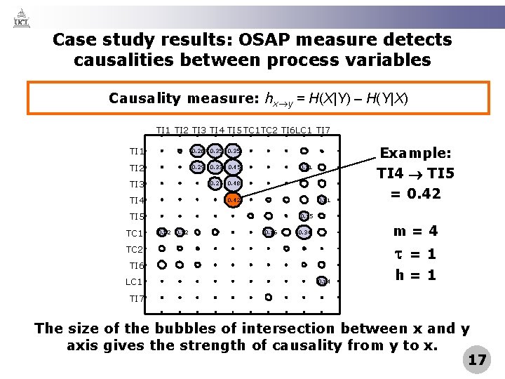
Case study results: OSAP measure detects causalities between process variables Causality measure: hx y = H(X|Y) – H(Y|X) TI 1 TI 2 TI 3 TI 4 TI 5 TC 1 TC 2 TI 6 LC 1 TI 7 TI 1 0. 28 0. 35 TI 2 0. 29 0. 33 0. 45 TI 3 0. 27 0. 48 TI 4 0. 42 0. 11 TI 5 TC 1 0. 15 0. 12 0. 16 m=4 0. 34 =1 TC 2 TI 6 LC 1 Example: TI 4 TI 5 = 0. 42 0. 14 h=1 TI 7 The size of the bubbles of intersection between x and y axis gives the strength of causality from y to x. 17

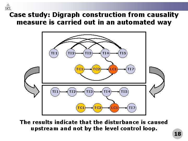
Case study: Digraph construction from causality measure is carried out in an automated way TI 1 TI 2 TI 3 TC 1 TI 2 TI 4 TC 2 TI 3 TC 1 TI 5 LC 1 TI 4 TC 2 TI 7 TI 5 LC 1 TI 7 The results indicate that the disturbance is caused upstream and not by the level control loop. 18

Agenda Motivation Method Case Study Conclusion 19

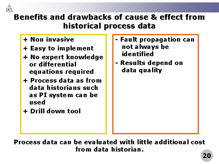
Benefits and drawbacks of cause & effect from historical process data + Non invasive + Easy to implement + No expert knowledge or differential equations required + Process data as from data historians such as PI system can be used + Drill down tool - Fault propagation can not always be identified - Results depend on data quality Process data can be evaluated with little additional cost from data historian. 20

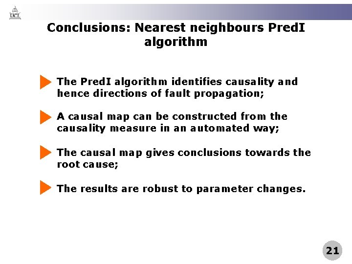
Conclusions: Nearest neighbours Pred. I algorithm The Pred. I algorithm identifies causality and hence directions of fault propagation; A causal map can be constructed from the causality measure in an automated way; The causal map gives conclusions towards the root cause; The results are robust to parameter changes. 21