MEASURES OF DISPERSION SPREAD AND VARIABILITY DATA SETS

MEASURES OF DISPERSION: SPREAD AND VARIABILITY

DATA SETS FOR PROJECT • NES 2000. sav • States. sav • World. sav

Outline: Key Measures of Dispersion (Interval Scale) 1. Range 2. Variance 3. Standard Deviation 4. Standard Score

1. Range of Values Xmax – Xmin = Range

i i

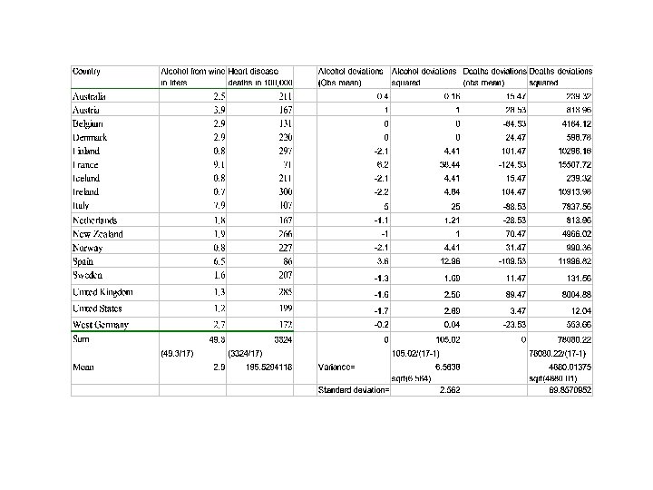
2. The Meaning of Variance Formula: Variance = s 2 = Σ (Xi – X)2/n [or n – 1] Definition: Mean squared deviation from the mean That is: Overall variation or cumulative “spread” of values around the arithmetic mean (or “average”) for a variable Relevance: A key goal of statistical analysis is to detect underlying patterns within the overall variance. Question: Why are some values below the mean and some values above? Can we find an explanation?

2. Variance (continued) • Thus: We want to understand variation in values of a variable—the so-called “dependent” variable. • Question: Might the variation in the dependent variable be a function (or consequence) of variation in another variable—the “independent” variable? • Key concept: Explanation of variance (in the dependent variable).

3. The Standard Deviation • Measure of how individual observations deviate from or vary around the mean of the variable • Allows comparison of variation: – Standard deviation is 0 only if no variation – The greater the spread, the greater the standard deviation of variable – Two variables with similar means but different standard deviations differ in extent of variation around mean

4. Standard Scores (Z Scores) • Definition: Zi = (Xi – X)/s • Measures distance from mean in standard deviation units • Allows comparison across variables • Useful in construction of composite variables (i. e. , adding apples and oranges—or level of education plus annual income, or GDP per capita plus life expectancy)

Reprise: Constructing Composite Indicators--Two Key Problems • 1. Aggregating Indicators • Add, multiply…. ? • Apples and oranges? • 2. Weighting Indicators • Are some indicators “more important”? • Weighting cannot be avoided

Example: Socio-economic Status • Education: Mean = 10 years , sd = 2, observation X = 16, Zx = (16 -10)/2 = + 3 • Parents’ annual income: Mean = $ 50, 000, sd = 5, 000, observation X = $40, 000, Zx = (40, 000 -50, 000)/5, 000 = -2

Alternative Results Composite scale 1/Mobility and Class Equal Z 1 = 3 + (-2) = + 1 Composite scale 2/Social Mobility>Class Z 2 = 3(2) + (-2) = + 4 Composite scale 3/Economic Class>Mobility Z 3 = 3 + 2(-2) = -1

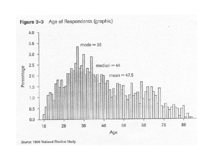
Postscript: On Skewness Sk = (X – Mo)/s = 3 (X – Md)/s Sk = 0 for a symmetrical (normal) curve, positive if skewed to the right, negative if skewed to the left If Sk > 1, consider using median not mean If Sk/standard error >2, use median not mean