MEASURES OF CENTRAL TENDENCY AVERAGES Topic 6 Measures

MEASURES OF CENTRAL TENDENCY (AVERAGES) Topic #6

Measures of Central Tendency • A measure of central tendency is a univariate statistic that indicates, in one manner or another, – the average or typical observed value of a variable in a data set, or – put otherwise, the center of the frequency distribution of the data.

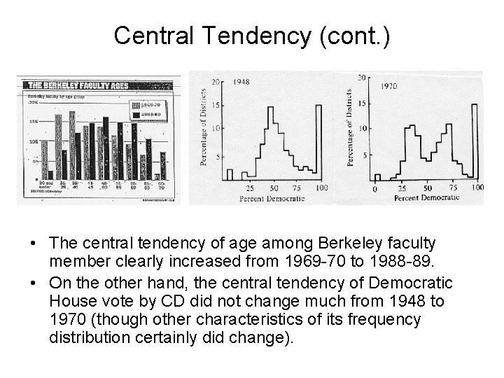
Central Tendency (cont. ) • The central tendency of age among Berkeley faculty member clearly increased from 1969 -70 to 1988 -89. • On the other hand, the central tendency of Democratic House vote by CD did not change much from 1948 to 1970 (though other characteristics of its frequency distribution certainly did change).

How to Calculate Averages • We consider three measures of central tendency that are appropriate for three different levels of measurement (nominal, ordinal, and interva). – There are others, e. g. , the geometric and harmonic means, appropriate only for ratio variables. • For each measure of central tendency, we will consider how it may be calculated from three different “starting points”: – a list of observed values (i. e. , raw data, e. g. , one column in a data spread sheet); – a frequency table (or bar graph); – a histogram and, in particular, a • continuous density curve (like income in PS #5 C).

The Mode • The mode (or modal value) of a variable in a set of data is the value of the variable that is observed most frequently in that data (or, given a continuous frequency curve, is at the point of greatest density). – Note: the mode is the value that is observed most frequently, not the frequency itself. (I see this error too frequently on tests. ) • The mode is defined for every type of variable [i. e. , nominal, ordinal, interval, or ratio]. – However, the mode is used as a measure of central tendency primarily for nominal variables only.

The Mode (cont. ) • The mode is defined for ordinal and interval variables as well. • But since it takes account of only the nominal characteristics of variables (i. e. , whether two cases have the same or different values), it is usually very unsatisfactory when applied to ordinal or higher level variables. – The mode may be ill-defined if we have either: • a small number of cases; or • a precisely measured continuous variable and a finite number of cases; – because in either event it is likely that no value will be observed more than once in the data. • In any event, the mode is unstable in that – small changes in the data can result in large and erratic changes in the modal value; and – changes in coding the variable (for example, RELIGION), or changes in class intervals, can change the modal value.

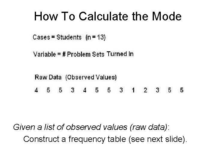
How To Calculate the Mode Given a list of observed values (raw data): Construct a frequency table (see next slide).

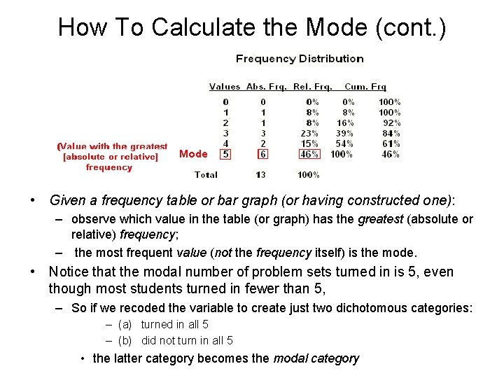
How To Calculate the Mode (cont. ) • Given a frequency table or bar graph (or having constructed one): – observe which value in the table (or graph) has the greatest (absolute or relative) frequency; – the most frequent value (not the frequency itself) is the mode. • Notice that the modal number of problem sets turned in is 5, even though most students turned in fewer than 5, – So if we recoded the variable to create just two dichotomous categories: – (a) turned in all 5 – (b) did not turn in all 5 • the latter category becomes the modal category

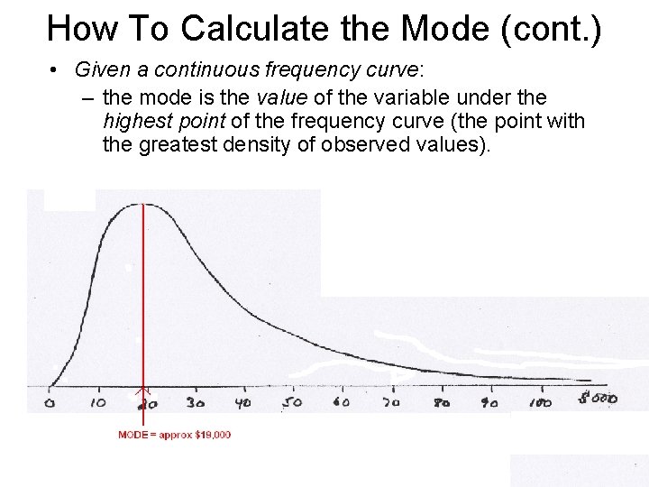
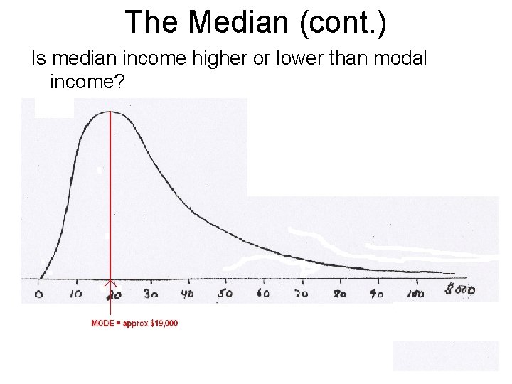
How To Calculate the Mode (cont. ) • Given a continuous frequency curve: – the mode is the value of the variable under the highest point of the frequency curve (the point with the greatest density of observed values).

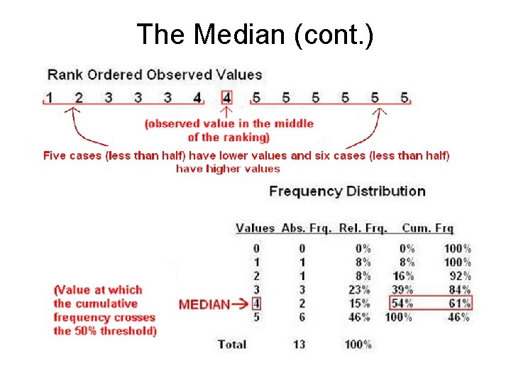
The Median • The median (or median value) of a variable in a data set is – the value in the middle of the observations, in the sense that no more than half of the cases have lower values and no more than half of the cases have higher values or, – more generally, such that no more than half of the cases have values that lie on either side of the median value. • Given a quite precisely measured continuous variable and a very large number of cases, we can in practice say that – half the cases have lower values and half have higher values (e. g. , LEVEL OF INCOME, SAT scores). – Equivalently, the median value is the value of the case at the 50 th percentile of the distribution.

The Median (cont. ) • The median is defined if and only if the variable is at least ordinal in nature [i. e. , ordinal, interval, or ratio], and we can therefore rank all (non-missing) observations in terms of lower to higher values (or possibly some other natural [e. g. , liberal to conservative] ordering). – e. g. , the median member of House of Representatives with respect to ideology: half are more liberal, half more conservative. • The median should be clearly distinguished from another (infrequently used) measure of central tendency that is defined only for variables that are interval in nature. – This is the midrange (or midpoint) value in the distribution, which is • the value in the middle of the observations in the (different) sense that it lies exactly halfway between the minimum (lowest) and maximum (highest) observed values (i. e. , at the midpoint of the range of values), i. e. , (min + max) / 2, • e. g. , for Problem Sets, (1 + 5) / 2 = 3

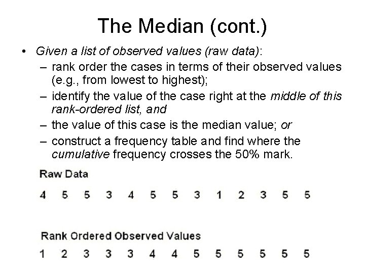
The Median (cont. ) • Given a list of observed values (raw data): – rank order the cases in terms of their observed values (e. g. , from lowest to highest); – identify the value of the case right at the middle of this rank-ordered list, and – the value of this case is the median value; or – construct a frequency table and find where the cumulative frequency crosses the 50% mark.

The Median (cont. )

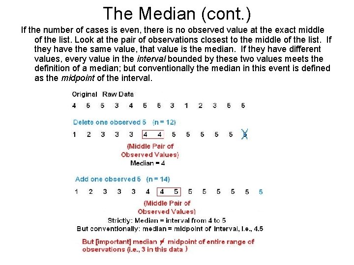
The Median (cont. ) If the number of cases is even, there is no observed value at the exact middle of the list. Look at the pair of observations closest to the middle of the list. If they have the same value, that value is the median. If they have different values, every value in the interval bounded by these two values meets the definition of a median; but conventionally the median in this event is defined as the midpoint of the interval.

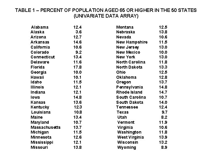
TABLE 1 – PERCENT OF POPULATION AGED 65 OR HIGHER IN THE 50 STATES (UNIVARIATE DATA ARRAY) Alabama Alaska Arizona Arkansas California Colorado Connecticut Delaware Florida Georgia Hawaii Idaho Illinois Indiana Iowa Kansas Kentucky Louisiana Maine Maryland Massachusetts Michigan Minnesota Mississippi Missouri 12. 4 3. 6 12. 7 14. 6 10. 6 9. 2 13. 4 11. 6 17. 8 10. 0 10. 1 11. 5 12. 1 14. 8 13. 6 12. 3 10. 8 13. 4 10. 7 13. 7 11. 5 12. 6 12. 1 13. 8 Montana Nebraska Nevada New Hampshire New Jersey New Mexico New York North Carolina North Dakota Ohio Oklahoma Oregon Pennsylvania Rhode Island South Carolina South Dakota Tennessee Texas Utah Vermont Virginia Washington West Virginia Wisconsin Wyoming 12. 5 13. 8 10. 6 11. 5 13. 0 10. 0 13. 0 11. 8 13. 3 12. 5 12. 8 13. 7 14. 8 14. 7 10. 7 14. 0 12. 4 9. 7 8. 2 11. 9 10. 6 11. 8 13. 9 13. 2 8. 9

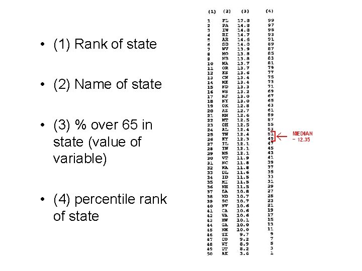
• (1) Rank of state • (2) Name of state • (3) % over 65 in state (value of variable) • (4) percentile rank of state

The Median (cont. ) Is median income higher or lower than modal income?

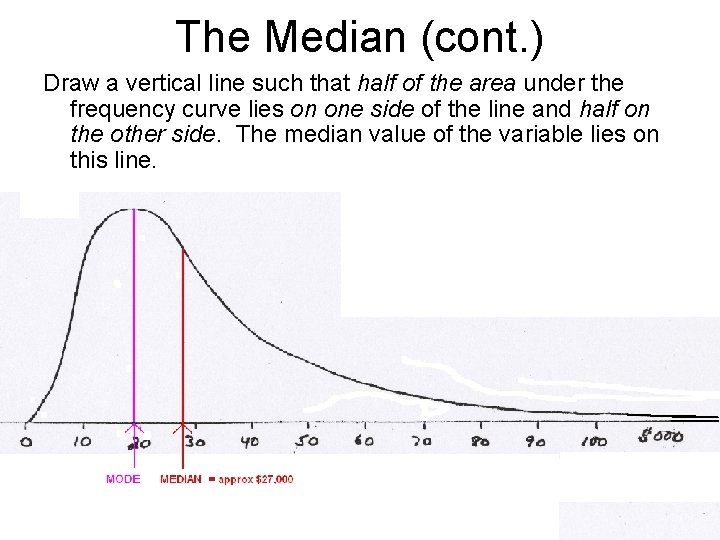
The Median (cont. ) Draw a vertical line such that half of the area under the frequency curve lies on one side of the line and half on the other side. The median value of the variable lies on this line.

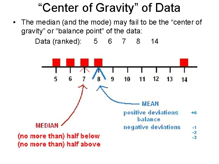
“Center of Gravity” of Data • The median (and the mode) may fail to be the “center of gravity” or “balance point” of the data: Data (ranked): 5 6 7 8 14

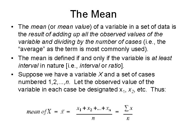
The Mean • The mean (or mean value) of a variable in a set of data is the result of adding up all the observed values of the variable and dividing by the number of cases (i. e. , the “average” as the term is most commonly used). • The mean is defined if and only if the variable is at least interval in nature [i. e. , interval or ratio]. • Suppose we have a variable X and a set of cases numbered 1, 2, . . . , n. Let the observed value of the variable in each case be designated x 1, x 2, etc. Thus:

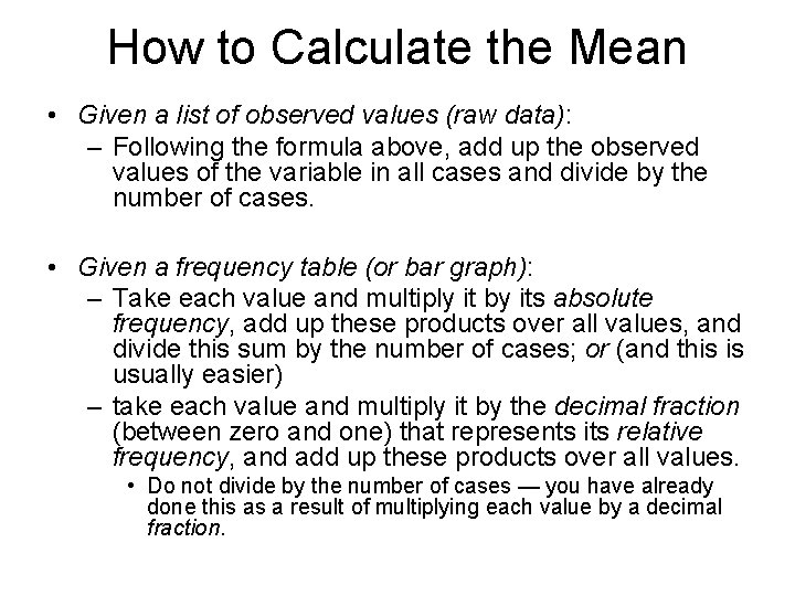
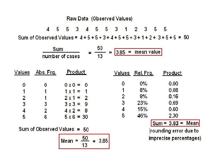
How to Calculate the Mean • Given a list of observed values (raw data): – Following the formula above, add up the observed values of the variable in all cases and divide by the number of cases. • Given a frequency table (or bar graph): – Take each value and multiply it by its absolute frequency, add up these products over all values, and divide this sum by the number of cases; or (and this is usually easier) – take each value and multiply it by the decimal fraction (between zero and one) that represents its relative frequency, and add up these products over all values. • Do not divide by the number of cases — you have already done this as a result of multiplying each value by a decimal fraction.

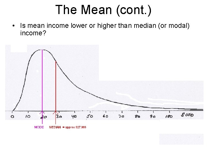
The Mean (cont. ) • Is mean income lower or higher than median (or modal) income?

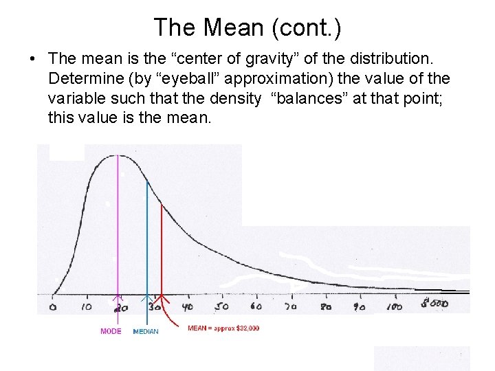
The Mean (cont. ) • The mean is the “center of gravity” of the distribution. Determine (by “eyeball” approximation) the value of the variable such that the density “balances” at that point; this value is the mean.

Average Values • For a quantitative variable, the range of observed values of a variable in a set of data is the interval extending from the minimum observed value to the maximum observed value. • For every measure of central tendency, the average value of the observations lies somewhere in this range, often (but certainly not always) somewhere near the middle of this range. – The modal or median observed value can equal the minimum or (like the modal problem sets turned in) the maximum value, but – the mean observation can do so only in the very special case in which all cases have identical observed values, so there is no dispersion [next topic] in the data and min value = max value. – Once again, remember that the median is not (necessarily) the midpoint of the range.

Average Values (cont. ) • If a quantitative variable is discrete, so all of its values are whole numbers, – the modal or median observed value is always a whole number also (with the possible exception noted for the median when the number of cases is even), but – the mean observation is almost never a whole number. – The “average” family may have 2. 374 children, • i. e. , the mean number of children per family may be 2. 374, • even though no individual family can have that [or any fractional] number of children. – Likewise, the mean number of problem sets turned in was 3. 85.

Deviations From the Average • Unless all cases have the same observed value [i. e. , no dispersion], some (in the case of mean, probably all) observed values will differ from the average value. • If the variable is interval (or ratio) in nature, we can calculate the deviation from the average in each case, – i. e. , the “distance” or “interval” from the observed value to the average value. • The deviation in each case is – positive if the observed value is greater than the average value, – negative if the observed value is less than the average value, or – zero if the observed value is equal to the average value.

Deviations From the Average (cont. ) • Since we have three different types of averages, we also have three different types of deviations from the average. The deviations from each type of average have different properties. – There are fewer non-zero deviations from the modal value than from any other value of the variable. – No more than half of the deviations from the median value are positive and no more than half are negative. – Unless several cases have the median value (and perhaps even then), the number of cases with positive deviations equals the number with negative deviations; that is, • the cases with positive and negative deviations balance out with respect to their number.

Deviations From the Average (cont. ) • The sum (or mean) of the absolute deviations (i. e. , ignoring whether the deviations are positive or negative) from the median is less than the sum (or mean) of the absolute deviations from any other value of the variable. • The sum (or mean) of the (“algebraic, ” i. e. , taking account of whether deviations are positive or negative) deviations from the mean is zero; that is, – the positive and negative deviations balance out with respect to their total (positive and negative) magnitudes. • The sum (or mean) of the squared deviations from the mean is less than the sum of the squared deviations from any other value of the variable.

Median vs. Mean Values • The mode is rarely used to describe central tendency in quantitative data, because (as we saw) it may be undefined or unstable. • Both the mean and the median are commonly used with quantitative (i. e. , interval or ratio) data, – though only the median can be used with ordinal data. – For example, it is common to report both median and mean income or wealth, median and mean test scores, median and mean prices (of cars, houses, etc. ). • While the median and the mean are both proper and useful measures of central tendency for quantitative variables, they have different definitions and properties and may (depending on the distribution of the data) give very different answers to the question “what is the average value in this data? ”

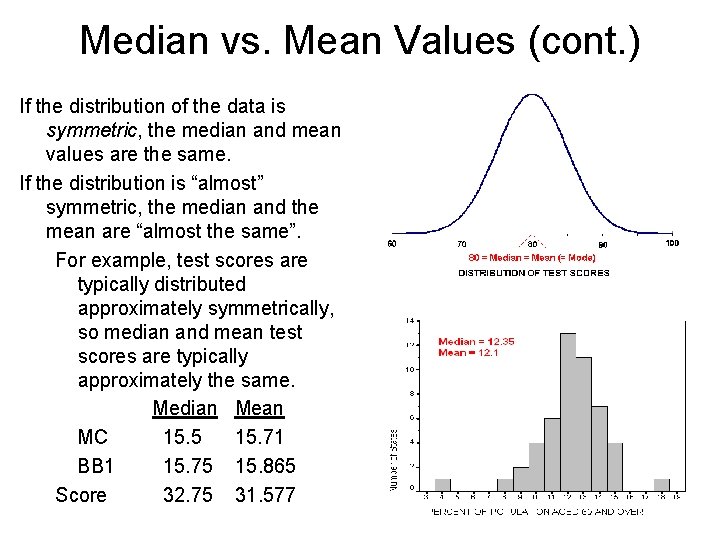
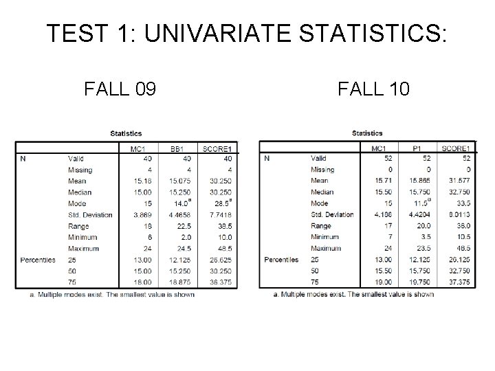
Median vs. Mean Values (cont. ) If the distribution of the data is symmetric, the median and mean values are the same. If the distribution is “almost” symmetric, the median and the mean are “almost the same”. For example, test scores are typically distributed approximately symmetrically, so median and mean test scores are typically approximately the same. Median Mean MC 15. 5 15. 71 BB 1 15. 75 15. 865 Score 32. 75 31. 577

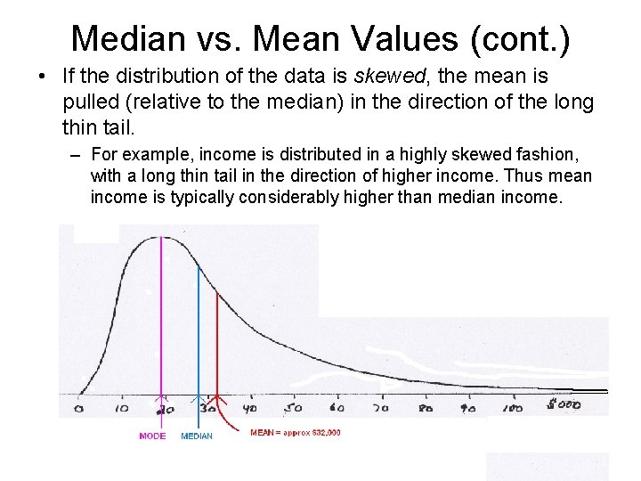
Median vs. Mean Values (cont. ) • If the distribution of the data is skewed, the mean is pulled (relative to the median) in the direction of the long thin tail. – For example, income is distributed in a highly skewed fashion, with a long thin tail in the direction of higher income. Thus mean income is typically considerably higher than median income.

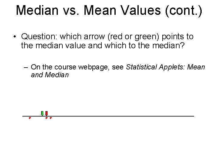
Median vs. Mean Values (cont. ) • Question: which arrow (red or green) points to the median value and which to the median? – On the course webpage, see Statistical Applets: Mean and Median

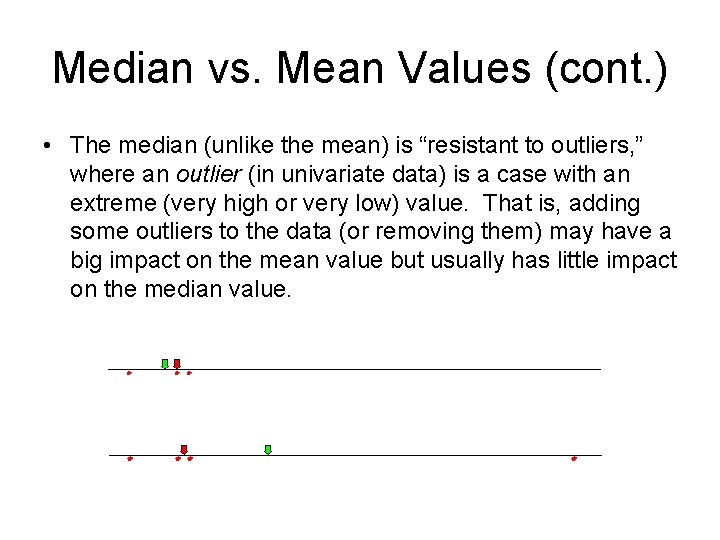
Median vs. Mean Values (cont. ) • The median (unlike the mean) is “resistant to outliers, ” where an outlier (in univariate data) is a case with an extreme (very high or very low) value. That is, adding some outliers to the data (or removing them) may have a big impact on the mean value but usually has little impact on the median value.

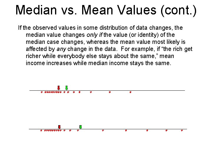
Median vs. Mean Values (cont. ) If the observed values in some distribution of data changes, the median value changes only if the value (or identity) of the median case changes, whereas the mean value most likely is affected by any change in the data. For example, if “the rich get richer while everybody else stays about the same, ” mean income increases while median income stays the same.

Median vs. Mean Values (cont. ) • If changes in the data do not change the sum of all observed values, i. e. , if the sum of all values remains constant, the mean remains constant, while the median may change. • For example, if Congress has decided that a tax cut will total $100 billion but has not decided how this fixed sum should be divided up among the nation’s 100 million households, • the median benefit will depend on the specifics of the legislation • but the mean tax benefit per household will be $1000 in any event.

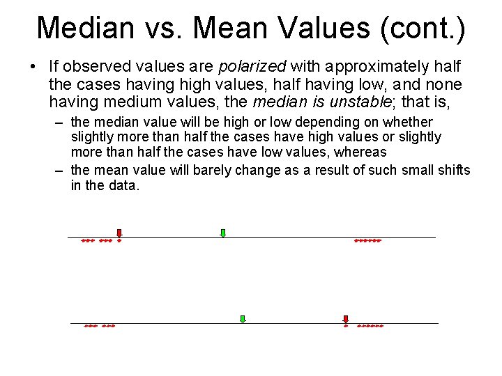
Median vs. Mean Values (cont. ) • If observed values are polarized with approximately half the cases having high values, half having low, and none having medium values, the median is unstable; that is, – the median value will be high or low depending on whether slightly more than half the cases have high values or slightly more than half the cases have low values, whereas – the mean value will barely change as a result of such small shifts in the data.

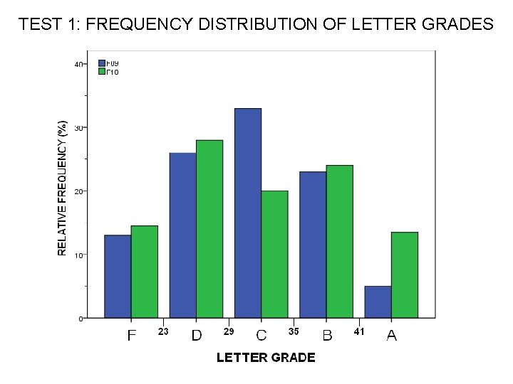
TEST 1: FREQUENCY DISTRIBUTION OF LETTER GRADES

TEST 1: UNIVARIATE STATISTICS: FALL 09 FALL 10

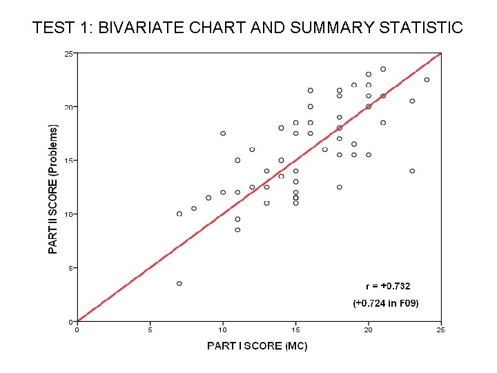
TEST 1: BIVARIATE CHART AND SUMMARY STATISTIC