Measures of Average In casual terms average means

Measures of Average In casual terms, average means the most typical case, or the center of the distribution. Measures of average are also called measures of central tendency, and include the mean, median, mode, and midrange.

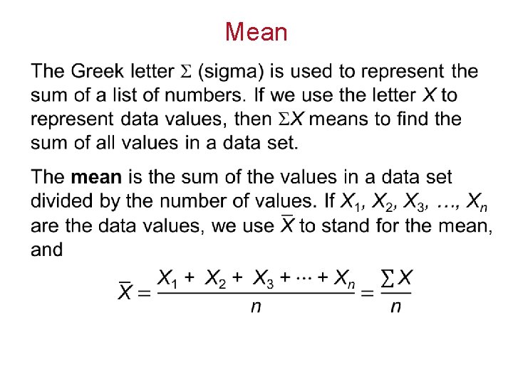
Mean •

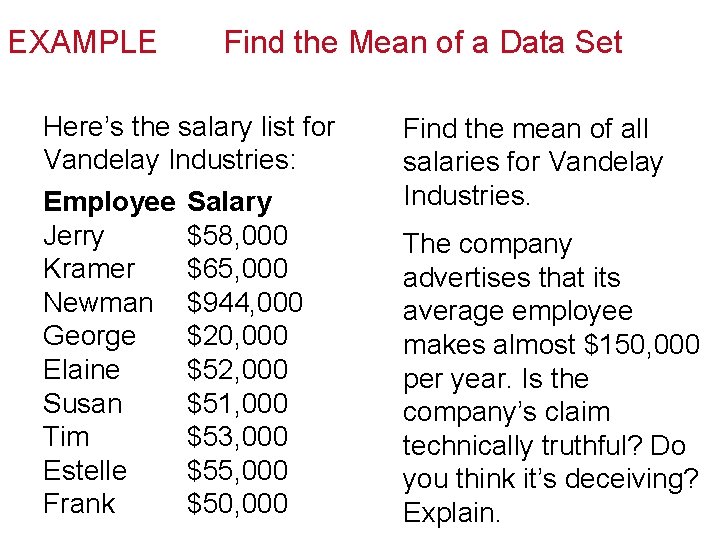
EXAMPLE Find the Mean of a Data Set Here’s the salary list for Vandelay Industries: Employee Salary Jerry $58, 000 Kramer $65, 000 Newman $944, 000 George $20, 000 Elaine $52, 000 Susan $51, 000 Tim $53, 000 Estelle $55, 000 Frank $50, 000 Find the mean of all salaries for Vandelay Industries. The company advertises that its average employee makes almost $150, 000 per year. Is the company’s claim technically truthful? Do you think it’s deceiving? Explain.

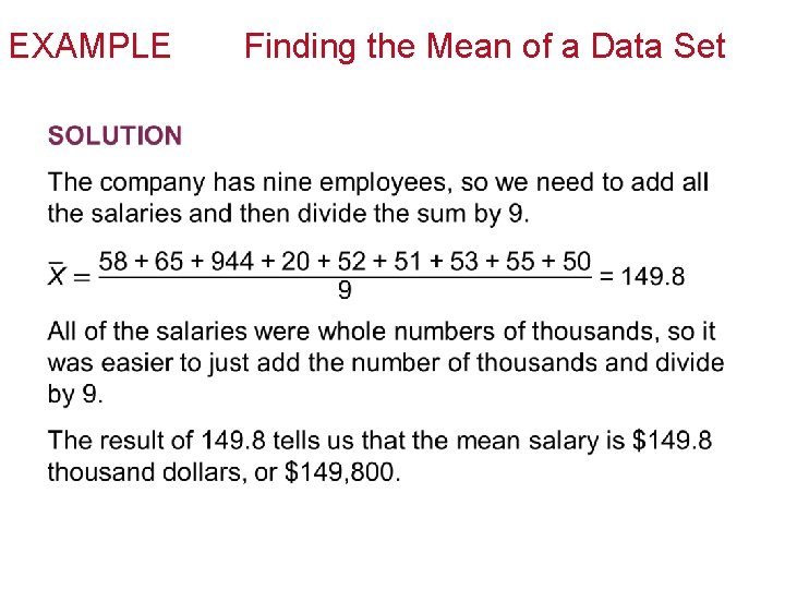
EXAMPLE • Finding the Mean of a Data Set

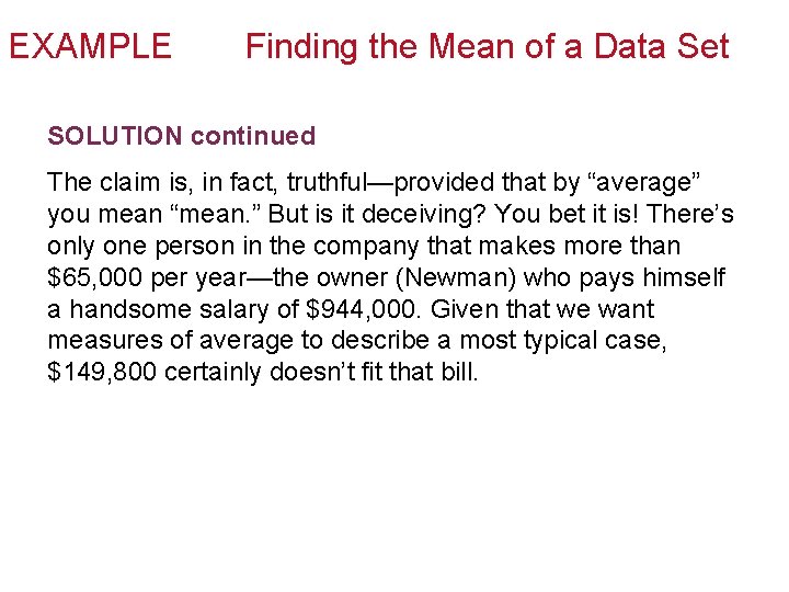
EXAMPLE Finding the Mean of a Data Set SOLUTION continued The claim is, in fact, truthful—provided that by “average” you mean “mean. ” But is it deceiving? You bet it is! There’s only one person in the company that makes more than $65, 000 per year—the owner (Newman) who pays himself a handsome salary of $944, 000. Given that we want measures of average to describe a most typical case, $149, 800 certainly doesn’t fit that bill.

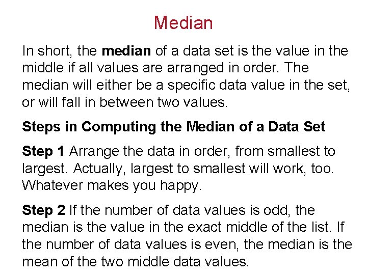
Median In short, the median of a data set is the value in the middle if all values are arranged in order. The median will either be a specific data value in the set, or will fall in between two values. Steps in Computing the Median of a Data Set Step 1 Arrange the data in order, from smallest to largest. Actually, largest to smallest will work, too. Whatever makes you happy. Step 2 If the number of data values is odd, the median is the value in the exact middle of the list. If the number of data values is even, the median is the mean of the two middle data values.

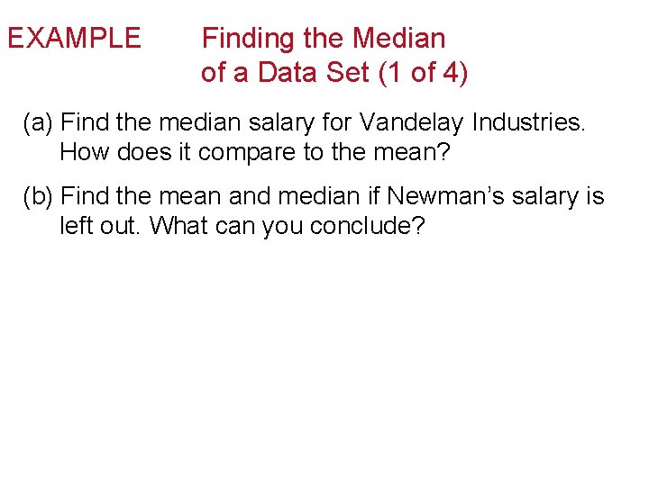
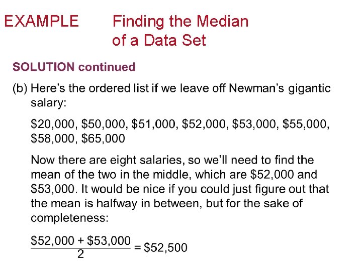
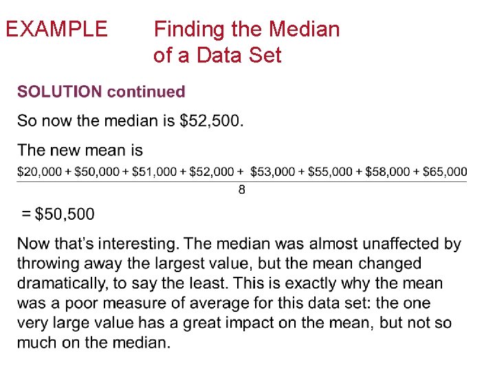
EXAMPLE Finding the Median of a Data Set (1 of 4) (a) Find the median salary for Vandelay Industries. How does it compare to the mean? (b) Find the mean and median if Newman’s salary is left out. What can you conclude?

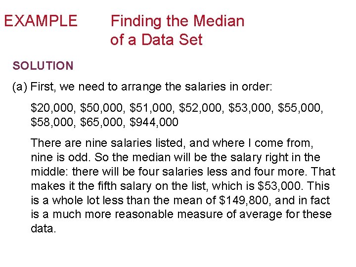
EXAMPLE Finding the Median of a Data Set SOLUTION (a) First, we need to arrange the salaries in order: $20, 000, $51, 000, $52, 000, $53, 000, $55, 000, $58, 000, $65, 000, $944, 000 There are nine salaries listed, and where I come from, nine is odd. So the median will be the salary right in the middle: there will be four salaries less and four more. That makes it the fifth salary on the list, which is $53, 000. This is a whole lot less than the mean of $149, 800, and in fact is a much more reasonable measure of average for these data.

EXAMPLE • Finding the Median of a Data Set

EXAMPLE • Finding the Median of a Data Set

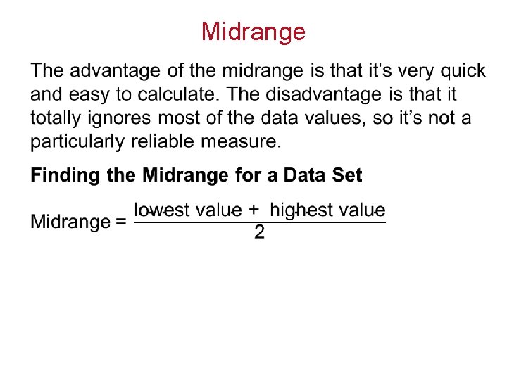
Midrange •

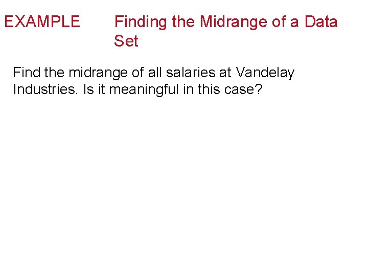
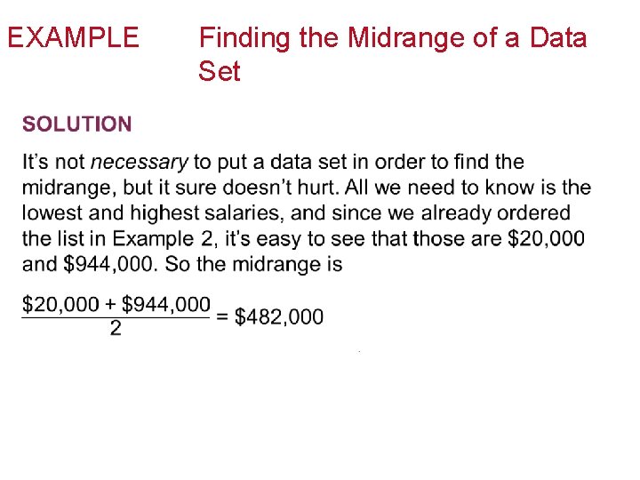
EXAMPLE Finding the Midrange of a Data Set Find the midrange of all salaries at Vandelay Industries. Is it meaningful in this case?

EXAMPLE • Finding the Midrange of a Data Set

Mode The mode is sometimes said to be the most typical case. The value that occurs most often in a data set is called the mode. A data set can have more than one mode or no mode at all.

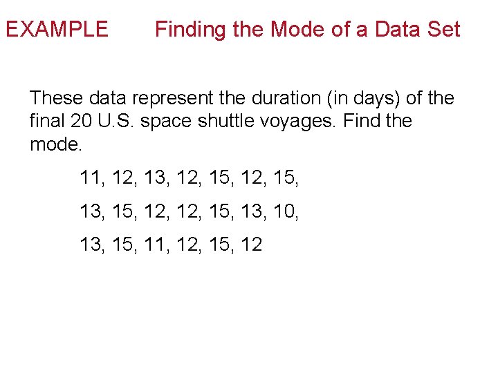
EXAMPLE Finding the Mode of a Data Set These data represent the duration (in days) of the final 20 U. S. space shuttle voyages. Find the mode. 11, 12, 13, 12, 15, 13, 15, 12, 15, 13, 10, 13, 15, 11, 12, 15, 12

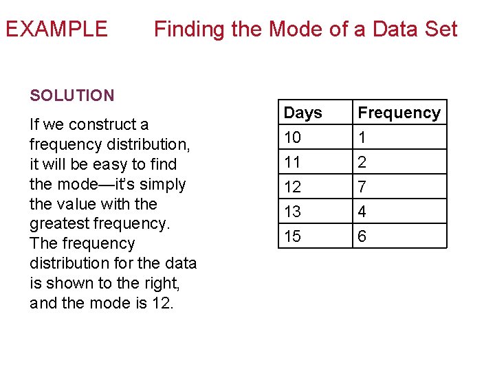
EXAMPLE Finding the Mode of a Data Set SOLUTION If we construct a frequency distribution, it will be easy to find the mode—it’s simply the value with the greatest frequency. The frequency distribution for the data is shown to the right, and the mode is 12. Days 10 11 12 13 15 Frequency 1 2 7 4 6

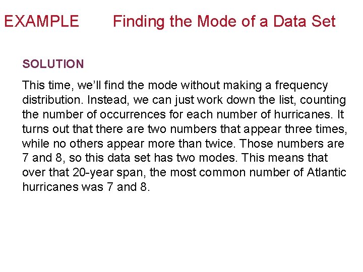
EXAMPLE Finding the Mode of a Data Set The number of Atlantic hurricanes for each of the years from 1997– 2016 is shown in the list. Find the mode, and describe what tells you. 3, 10, 8, 8, 9, 4, 7, 9, 15, 5, 6, 8, 3, 12, 7, 10, 2, 6, 4, 7

EXAMPLE Finding the Mode of a Data Set SOLUTION This time, we’ll find the mode without making a frequency distribution. Instead, we can just work down the list, counting the number of occurrences for each number of hurricanes. It turns out that there are two numbers that appear three times, while no others appear more than twice. Those numbers are 7 and 8, so this data set has two modes. This means that over that 20 -year span, the most common number of Atlantic hurricanes was 7 and 8.

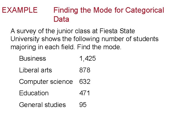
EXAMPLE Finding the Mode for Categorical Data A survey of the junior class at Fiesta State University shows the following number of students majoring in each field. Find the mode. Business 1, 425 Liberal arts 878 Computer science 632 Education 471 General studies 95

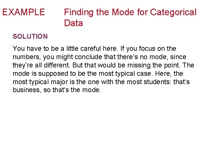
EXAMPLE Finding the Mode for Categorical Data SOLUTION You have to be a little careful here. If you focus on the numbers, you might conclude that there’s no mode, since they’re all different. But that would be missing the point. The mode is supposed to be the most typical case. Here, the most typical major is the one with the most students: that’s business, so that’s the mode.

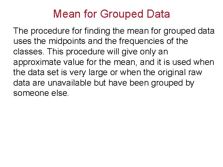
Mean for Grouped Data The procedure for finding the mean for grouped data uses the midpoints and the frequencies of the classes. This procedure will give only an approximate value for the mean, and it is used when the data set is very large or when the original raw data are unavailable but have been grouped by someone else.

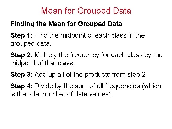
Mean for Grouped Data Finding the Mean for Grouped Data Step 1: Find the midpoint of each class in the grouped data. Step 2: Multiply the frequency for each class by the midpoint of that class. Step 3: Add up all of the products from step 2. Step 4: Divide by the sum of all frequencies (which is the total number of data values).

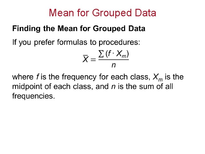
Mean for Grouped Data •

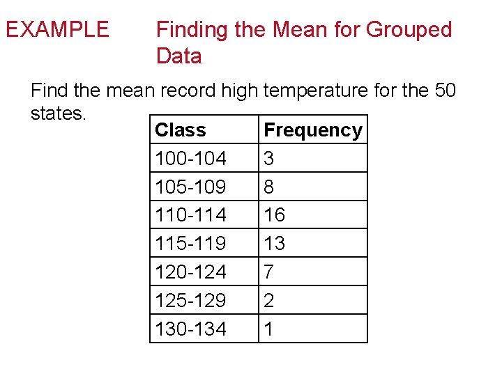
EXAMPLE Finding the Mean for Grouped Data Find the mean record high temperature for the 50 states. Class Frequency 100 -104 3 105 -109 8 110 -114 16 115 -119 13 120 -124 7 125 -129 2 130 -134 1

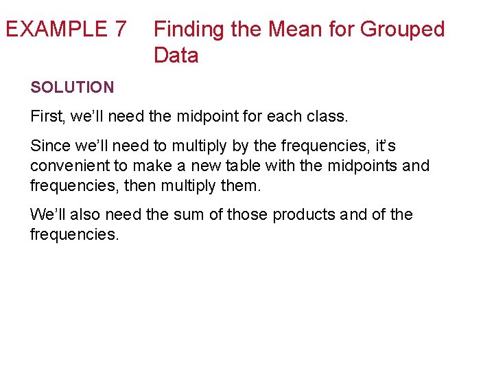
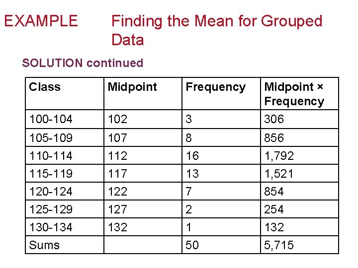
EXAMPLE 7 Finding the Mean for Grouped Data SOLUTION First, we’ll need the midpoint for each class. Since we’ll need to multiply by the frequencies, it’s convenient to make a new table with the midpoints and frequencies, then multiply them. We’ll also need the sum of those products and of the frequencies.

EXAMPLE Finding the Mean for Grouped Data SOLUTION continued Class Midpoint Frequency Midpoint × Frequency 100 -104 102 3 306 105 -109 110 -114 115 -119 120 -124 125 -129 130 -134 Sums 107 112 117 122 127 132 8 16 13 7 2 1 50 856 1, 792 1, 521 854 254 132 5, 715

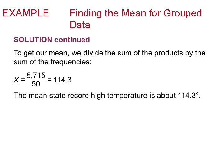
EXAMPLE • Finding the Mean for Grouped Data

EXAMPLE Comparing Measures of Average For the Vandelay Industries salary data, compare the four measures of average. Which do you think is the best description of the true average?

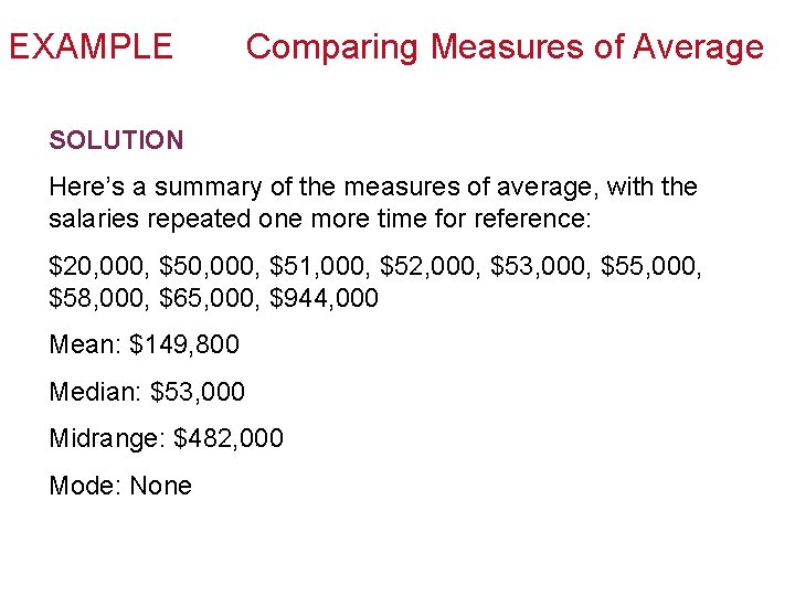
EXAMPLE Comparing Measures of Average SOLUTION Here’s a summary of the measures of average, with the salaries repeated one more time for reference: $20, 000, $51, 000, $52, 000, $53, 000, $55, 000, $58, 000, $65, 000, $944, 000 Mean: $149, 800 Median: $53, 000 Midrange: $482, 000 Mode: None

EXAMPLE Comparing Measures of Average SOLUTION continued Certainly the mode isn’t helpful for this data set. In fact, the only one that could possibly be considered as a reasonable average is the median. Aside from Newman’s $944 k, nobody makes more than $65, 000, so any “average” that’s more than twice that isn’t really a true reflection of the typical salary.

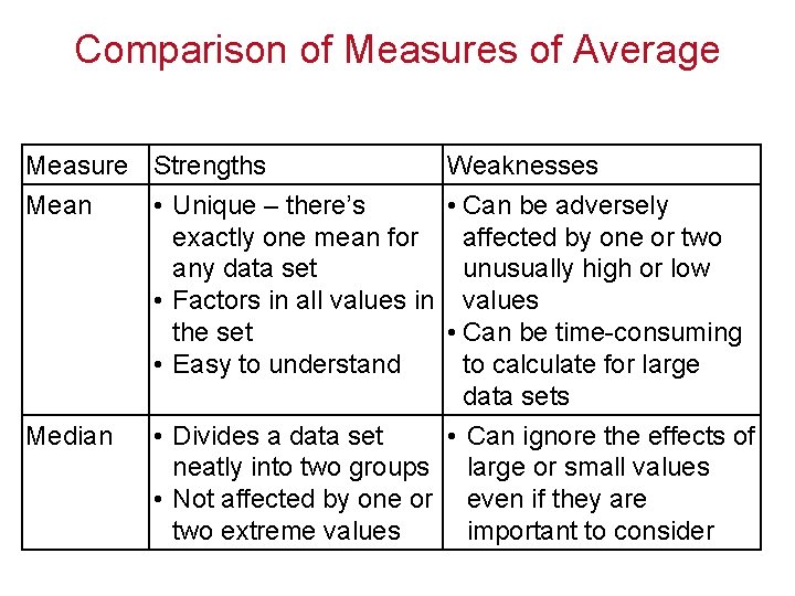
Comparison of Measures of Average Measure Strengths Weaknesses Mean • Unique – there’s • Can be adversely exactly one mean for affected by one or two any data set unusually high or low • Factors in all values in values the set • Can be time-consuming • Easy to understand to calculate for large data sets Median • Divides a data set • Can ignore the effects of neatly into two groups large or small values • Not affected by one or even if they are two extreme values important to consider

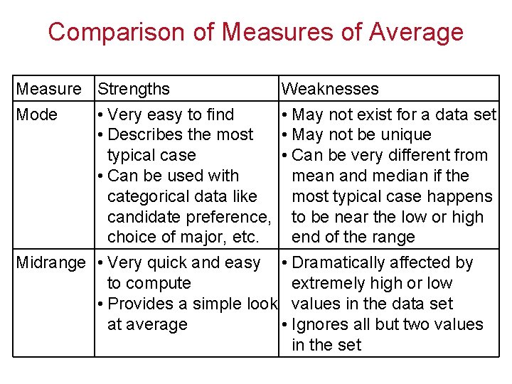
Comparison of Measures of Average Measure Strengths Weaknesses Mode • Very easy to find • May not exist for a data set • Describes the most • May not be unique typical case • Can be very different from • Can be used with mean and median if the categorical data like most typical case happens candidate preference, to be near the low or high choice of major, etc. end of the range Midrange • Very quick and easy • Dramatically affected by to compute extremely high or low • Provides a simple look values in the data set at average • Ignores all but two values in the set

Measures of Variation In this section we will study measures of variation, which will help to describe how the data within a set vary. The three most commonly used measures of variation are range, variance, and standard deviation.

Range The range of a data set is the difference between the highest and lowest values in the set. Range = Highest value – lowest value

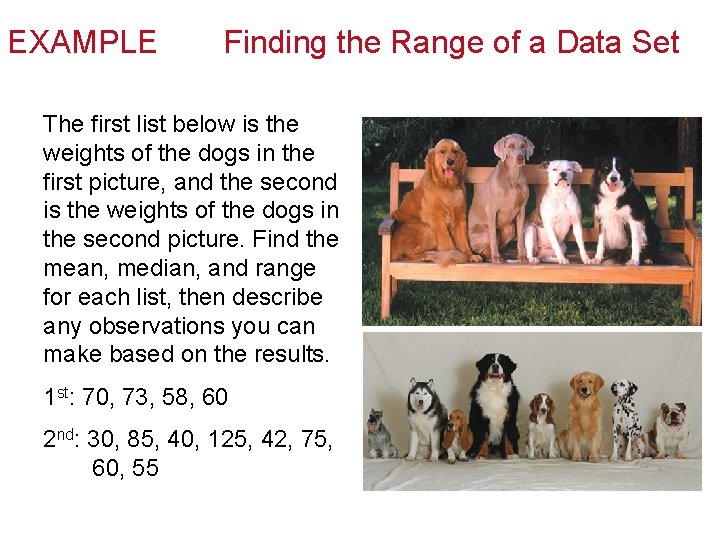
EXAMPLE Finding the Range of a Data Set The first list below is the weights of the dogs in the first picture, and the second is the weights of the dogs in the second picture. Find the mean, median, and range for each list, then describe any observations you can make based on the results. 1 st: 70, 73, 58, 60 2 nd: 30, 85, 40, 125, 42, 75, 60, 55

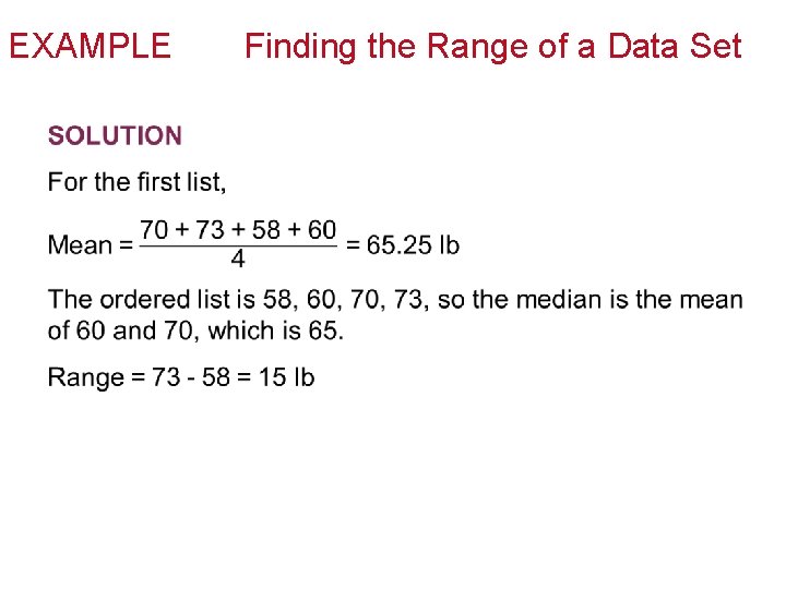
EXAMPLE • Finding the Range of a Data Set

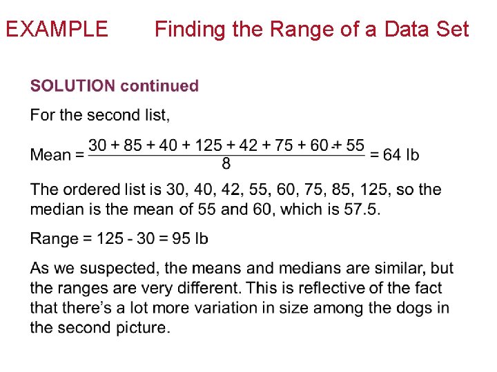
EXAMPLE • Finding the Range of a Data Set

Variance and Standard Deviation If most of the values are similar, but there’s just one unusually high value, the range will make it look like there’s a lot more variation than there actually is. For this reason, we will next define variance and standard deviation, which are much more reliable measures of variation.

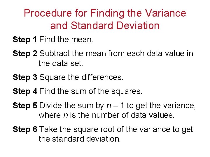
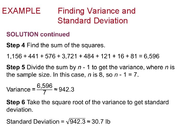
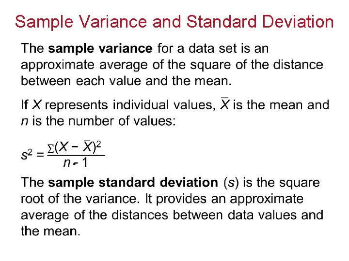
Procedure for Finding the Variance and Standard Deviation Step 1 Find the mean. Step 2 Subtract the mean from each data value in the data set. Step 3 Square the differences. Step 4 Find the sum of the squares. Step 5 Divide the sum by n – 1 to get the variance, where n is the number of data values. Step 6 Take the square root of the variance to get the standard deviation.

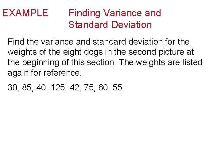
EXAMPLE Finding Variance and Standard Deviation Find the variance and standard deviation for the weights of the eight dogs in the second picture at the beginning of this section. The weights are listed again for reference. 30, 85, 40, 125, 42, 75, 60, 55

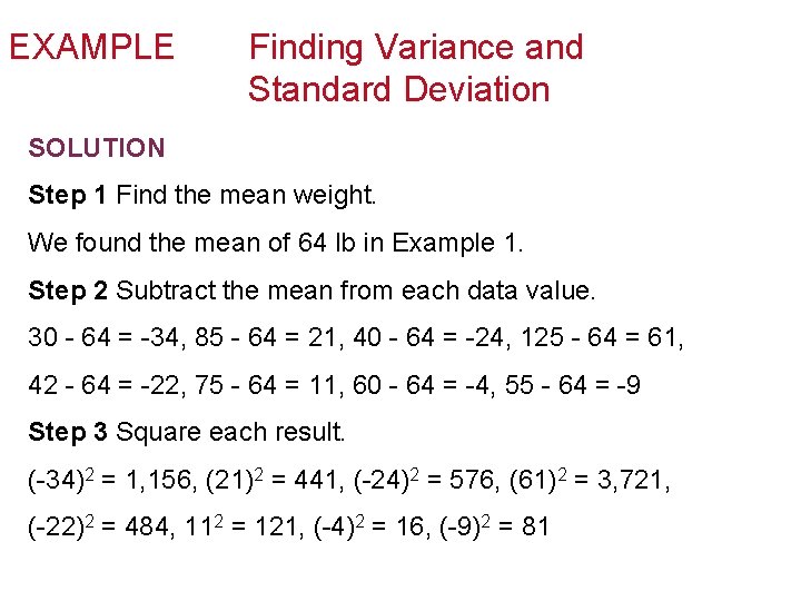
EXAMPLE Finding Variance and Standard Deviation SOLUTION Step 1 Find the mean weight. We found the mean of 64 lb in Example 1. Step 2 Subtract the mean from each data value. 30 - 64 = -34, 85 - 64 = 21, 40 - 64 = -24, 125 - 64 = 61, 42 - 64 = -22, 75 - 64 = 11, 60 - 64 = -4, 55 - 64 = -9 Step 3 Square each result. (-34)2 = 1, 156, (21)2 = 441, (-24)2 = 576, (61)2 = 3, 721, (-22)2 = 484, 112 = 121, (-4)2 = 16, (-9)2 = 81

EXAMPLE • Finding Variance and Standard Deviation

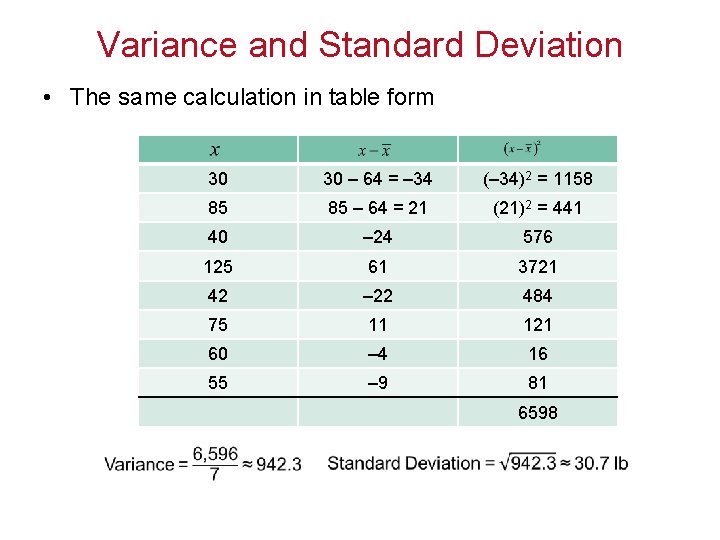
EXAMPLE Finding Variance and Standard Deviation SOLUTION continued To organize the steps, you might find it helpful to make a table with three columns: the original data, the difference between each data value and the mean, and their squares. Then you just add the entries in the last column and divide by n - 1 to get the variance.

Variance and Standard Deviation • The same calculation in table form 30 30 – 64 = – 34 (– 34)2 = 1158 85 85 – 64 = 21 (21)2 = 441 40 – 24 576 125 61 3721 42 – 22 484 75 11 121 60 – 4 16 55 – 9 81 6598

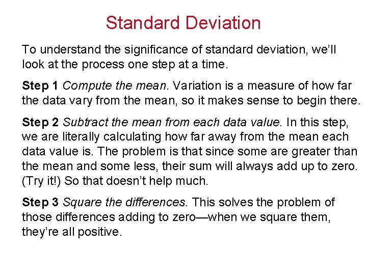
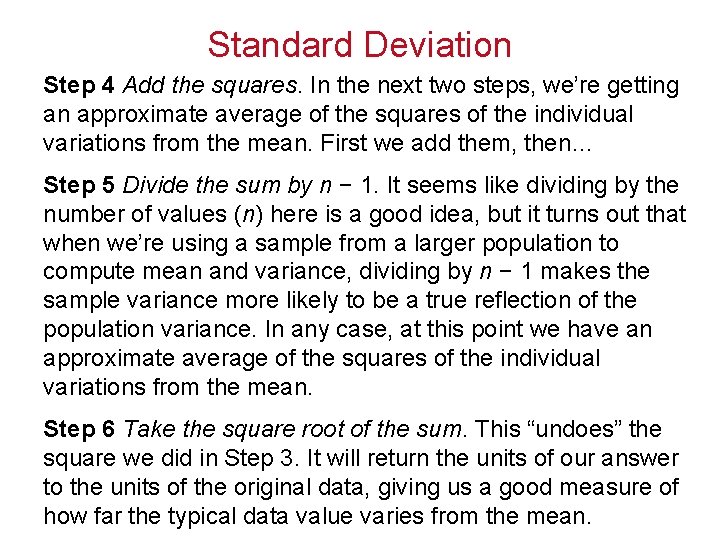
Standard Deviation To understand the significance of standard deviation, we’ll look at the process one step at a time. Step 1 Compute the mean. Variation is a measure of how far the data vary from the mean, so it makes sense to begin there. Step 2 Subtract the mean from each data value. In this step, we are literally calculating how far away from the mean each data value is. The problem is that since some are greater than the mean and some less, their sum will always add up to zero. (Try it!) So that doesn’t help much. Step 3 Square the differences. This solves the problem of those differences adding to zero—when we square them, they’re all positive.

Standard Deviation Step 4 Add the squares. In the next two steps, we’re getting an approximate average of the squares of the individual variations from the mean. First we add them, then… Step 5 Divide the sum by n − 1. It seems like dividing by the number of values (n) here is a good idea, but it turns out that when we’re using a sample from a larger population to compute mean and variance, dividing by n − 1 makes the sample variance more likely to be a true reflection of the population variance. In any case, at this point we have an approximate average of the squares of the individual variations from the mean. Step 6 Take the square root of the sum. This “undoes” the square we did in Step 3. It will return the units of our answer to the units of the original data, giving us a good measure of how far the typical data value varies from the mean.

Sample Variance and Standard Deviation •

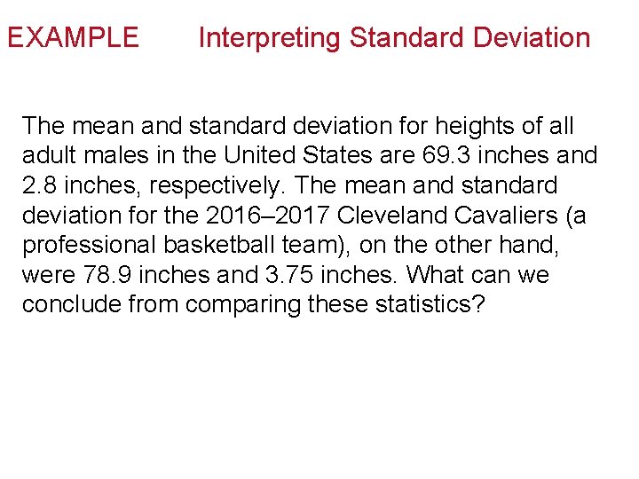
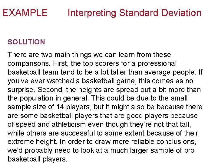
EXAMPLE Interpreting Standard Deviation The mean and standard deviation for heights of all adult males in the United States are 69. 3 inches and 2. 8 inches, respectively. The mean and standard deviation for the 2016– 2017 Cleveland Cavaliers (a professional basketball team), on the other hand, were 78. 9 inches and 3. 75 inches. What can we conclude from comparing these statistics?

EXAMPLE Interpreting Standard Deviation SOLUTION There are two main things we can learn from these comparisons. First, the top scorers for a professional basketball team tend to be a lot taller than average people. If you’ve ever watched a basketball game, this comes as no surprise. Second, the heights are spread out a bit more than the population in general. This could be due to the small sample size of 14 players, but it might also be because there are some basketball players that are good players because of speed and athleticism even though they’re not that tall, while others are successful to some extent because of their extreme height. In order to draw more reliable conclusions, we’d probably need to look at a much larger sample of pro basketball players.

EXAMPLE Interpreting Standard Deviation A professor has two sections of Math 115 this semester. The 8: 30 A. M. class has a mean score of 74% with a standard deviation of 3. 6%. The 2 P. M. class also has a mean score of 74%, but a standard deviation of 9. 2%. What can we conclude about the students’ averages in these two sections?

EXAMPLE Interpreting Standard Deviation SOLUTION In relative terms, the morning class has a small standard deviation and the afternoon class has a large one. So even though they have the same mean, the classes are quite different. In the morning class, most of the students probably have scores relatively close to the mean, with few very high or very low scores. In the afternoon class, the scores vary more widely, with a lot of high scores and a lot of low scores that average out to a mean of 74%.