Measurements Measurements and errors Here the goal is

Measurements • Measurements and errors : - Here , the goal is to have some understanding of the operation and behavior of electrical test instruments. Also , to gain practical information on their use.

• Instruments : is a device for determining the value or magnitude of a quantity or a variable. 1) Accuracy : is a measure of how close the output reading of an instrument is to the correct value. Note : In practice , it’s more usual to express it by inaccuracy which is the extent to which a reading might be wrong ( uncertainty ).

• Example : a voltmeter with a voltage range of ( 0 -10 V ) with uncertainty of ± 1 % of the full scale (f. s) reading. - Notice that when measuring 10 V (f. s) we obtain a reading of 9. 9 and when measuring 1 V we obtain a reading of 1. 1 V which had an inaccuracy of 10% in the other hand for the 10 V just 1%. - Hence , it is very important that instruments are chosen such that their range is appropriate to the value being measured.

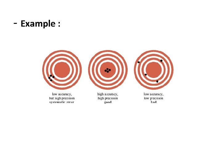
• 2) precision : it is a measure of the reproducibility of the reading that describes an instrument’s degree of agreement within a group of readings. This means that if a large numbers of reading are taken of the same quality by a high precision instrument , then the spread of readings will be very small.

• Note : High precision does not imply anything about measurement accuracy , ( a high precision instrument may have a low accuracy ). - The reproducibility describes the closeness of the output readings for the same input when there are changes in the method of measurement , observer , measuring instrument , location , conditions of use and time of measurement. - The reproducibility in measurements from an instrument is one way of expressing it’s precision.

- Example :

• 3) Sensitivity : it is the ratio of the output signal ( or response ) of the instrument to a change of input. • 4) Resolution : is the lowest limit on the magnitude of the change in the input measured quantity that produces an observable change in the instrument output.

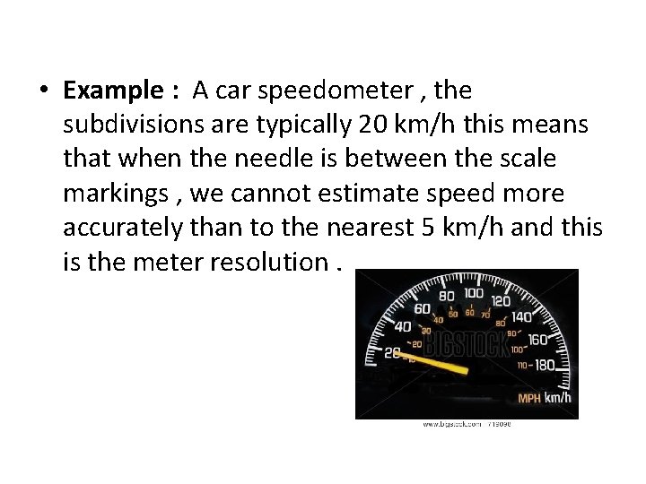
• Example : A car speedometer , the subdivisions are typically 20 km/h this means that when the needle is between the scale markings , we cannot estimate speed more accurately than to the nearest 5 km/h and this is the meter resolution.

5) Error : is the deviation from the true value of the measured variable. - Note : precision is composed by two things : - 1 - conformity ( necessary , but not a sufficient condition for precision (lack of significant figures ). 2 - significant figures. - Precision is a necessary , but not sufficient for accuracy.

• Significant figures : - None zero integers : they always count as significant figures. - Zeros : (a) Leading zeros : They never count as significant figures. Example : 0. 0025 2 S. F 0. 00250 3 S. F

(b) captive zeros : They always count as S. F. Example : 1. 008 4 S. F (c) Trailing zeros : These zeros are S. F only if the number contains a decimal point. Example : 100 1 S. F 100. 0 4 S. F 100. 3 S. F 1. 00 X 1020 3 S. F

- Note : The expression ( 1. 00 X 102 ) has some advantages : 1) The number of significant figures can be easily indicated. 2) Fewer zeros are needed to write a very large/small numbers.

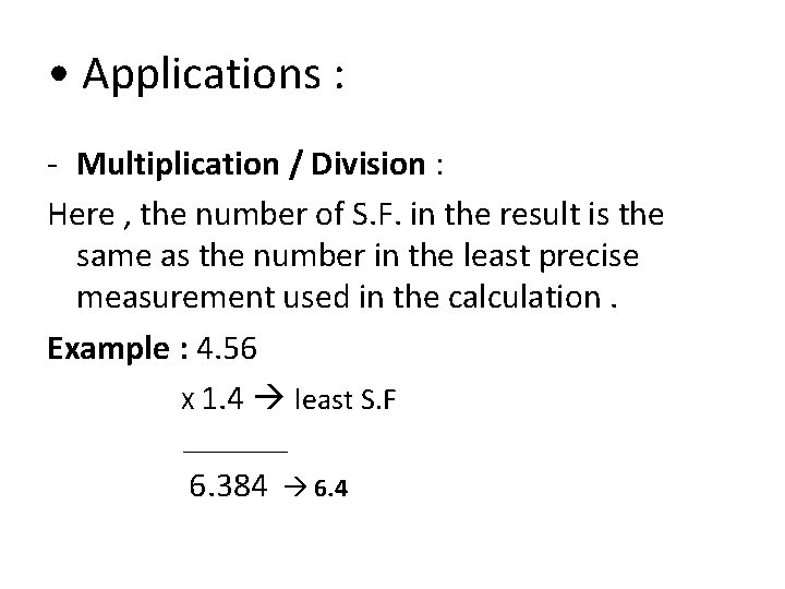
• Applications : - Multiplication / Division : Here , the number of S. F. in the result is the same as the number in the least precise measurement used in the calculation. Example : 4. 56 X 1. 4 least S. F ____ 6. 384 6. 4

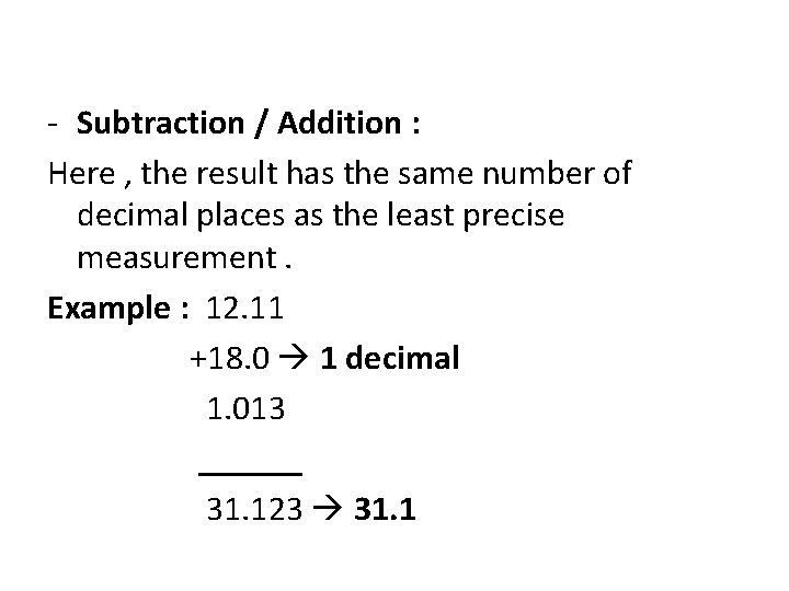
- Subtraction / Addition : Here , the result has the same number of decimal places as the least precise measurement. Example : 12. 11 +18. 0 1 decimal 1. 013 ______ 31. 123 31. 1

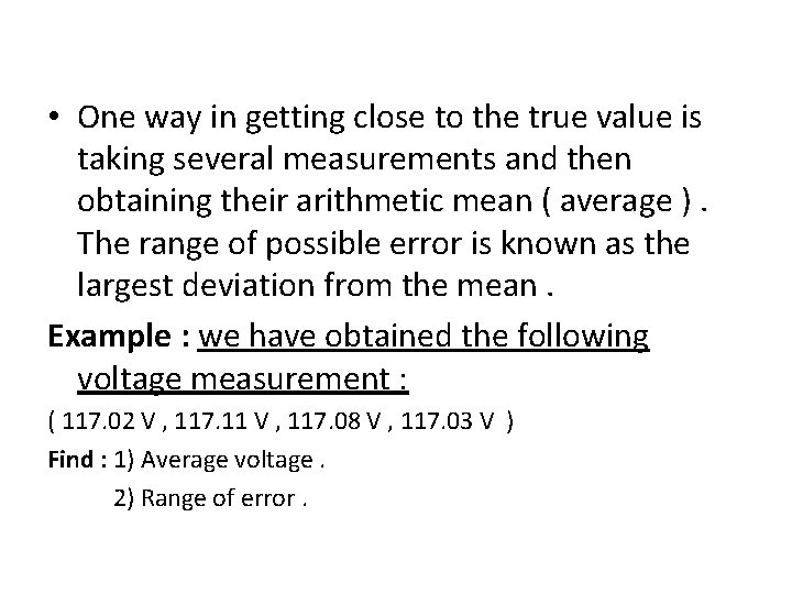
• One way in getting close to the true value is taking several measurements and then obtaining their arithmetic mean ( average ). The range of possible error is known as the largest deviation from the mean. Example : we have obtained the following voltage measurement : ( 117. 02 V , 117. 11 V , 117. 08 V , 117. 03 V ) Find : 1) Average voltage. 2) Range of error.

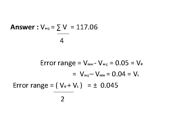
Answer : Vavg = ∑ V = 117. 06 ______ 4 Error range = Vmax - Vavg = 0. 05 = VH = Vavg – Vmin = 0. 04 = VL Error range = ( VH + VL ) = ± 0. 045 ___________ 2

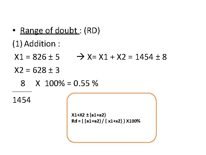
• Range of doubt : (RD) (1) Addition : X 1 = 826 ± 5 X= X 1 + X 2 = 1454 ± 8 X 2 = 628 ± 3 8 X 100% = 0. 55 % _________ 1454 X 1+X 2 ± (a 1+a 2) Rd = ( (a 1+a 2) / ( x 1+x 2) ) X 100%

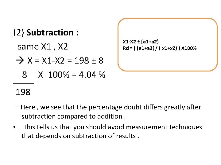
(2) Subtraction : same X 1 , X 2 X = X 1 -X 2 = 198 ± 8 8 X 100% = 4. 04 % X 1 -X 2 ± (a 1+a 2) Rd = ( (a 1+a 2) / ( x 1+x 2) ) X 100% _________ 198 - Here , we see that the percentage doubt differs greatly after subtraction compared to addition. • This tells us that you should avoid measurement techniques that depends on subtraction of results.

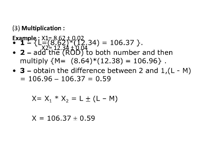
(3) Multiplication : • Example : X 1= 8. 62 ± 0. 02 X 2= 12. 34 ± 0. 04

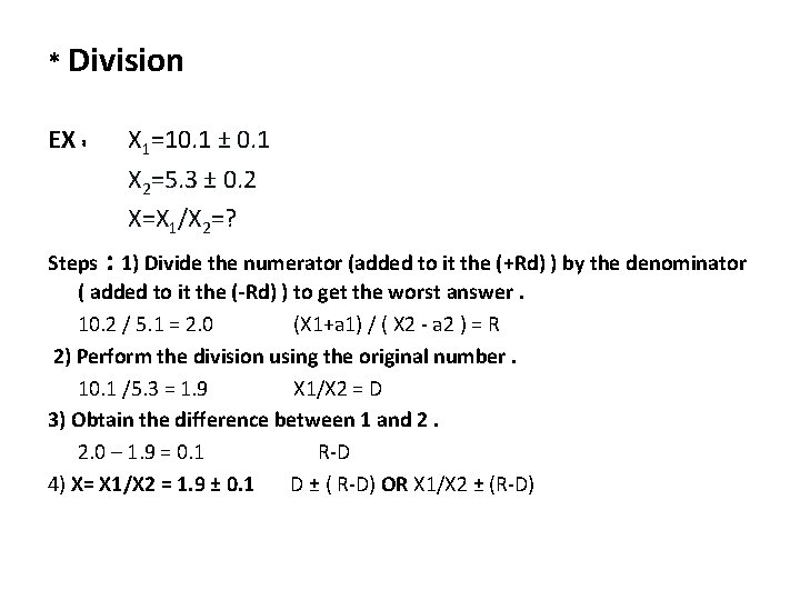
* Division EX : X 1=10. 1 ± 0. 1 X 2=5. 3 ± 0. 2 X=X 1/X 2=? Steps : 1) Divide the numerator (added to it the (+Rd) ) by the denominator ( added to it the (-Rd) ) to get the worst answer. 10. 2 / 5. 1 = 2. 0 (X 1+a 1) / ( X 2 - a 2 ) = R 2) Perform the division using the original number. 10. 1 /5. 3 = 1. 9 X 1/X 2 = D 3) Obtain the difference between 1 and 2. 2. 0 – 1. 9 = 0. 1 R-D 4) X= X 1/X 2 = 1. 9 ± 0. 1 D ± ( R-D) OR X 1/X 2 ± (R-D)

• Types of errors : In measurements , Errors may come from different sources : 1) Gross error : This error comes from human mistakes in reading or using the instrument. Example : A voltmeter with sensitivity of 1000 Ω/V reads 100 V on its 150 V scale when connected across an unknown resistor in series with a milliameter when it reads 5 m. A. 1) Apparent resistance of the unknown. 2) The actual resistance of the unknown. 3) Error due to the loading effect of the voltmeter.

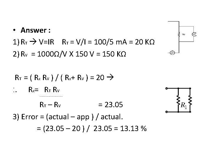
• Answer : 1) RT V=IR RT = V/I = 100/5 m. A = 20 KΩ 2) RV = 1000Ω/V X 150 V = 150 KΩ RT = ( Rx RV ) / ( Rx+ RV ) = 20 ׃. Rx= RT RV ---------------- RT – RV = 23. 05 3) Error = (actual – app ) / actual. = (23. 05 – 20 ) / 23. 05 = 13. 13 %

2) Systematic error : a) Instrumental error. b)Environmental error. a. This error is due to the instruments mechanical structures. ( i. e. calibration error ). Here , there is a need for setting the instrument at the zero reference before taking any measurement.

• Hence , in general : (1) One should select a suitable instrument. (2) Apply correction factor after determining the amount of instrument error. - One should check for erratic behavior and stability and reproducibility of result.

• b. Here, external conditions affecting the instrument (i. e. change in temperature , humidity, pressure , magnetic field … etc ). - The Instrumental error is subdivided into 2 categories : 1 - static : this error is cause by the limitation of the device. 2 - Dynamic : this error is caused by the instrument not responding fast enough to follow changes in the measured value.

• 3) Random error : Is an error that is caused by unknown causes. This error may occur even when systematic errors have been accounted for. Example : A voltmeter monitoring a voltage for half an hour , readings that vary slightly will be seen over the period of observation , the only way to offset ( overcomes) these errors is by increasing the number of readings and using the statistical mean.

• Arithmetic mean ( average ) : It represents the most probable value of a measured variable. The more readings we have, the more accurate results we get.