Mean shift A segmentation and tracking algorithm http


 denote a kernel function that indicates how much point x")


: density estimate")
. �Initialize windows at")


} and ρ(p(z) , q)")

} and ρ(p(z) , q). 5. While ρ(p(z) ,")
} and ρ(p(z) , q). 5. While ρ(p(z) ,")

 Frame 1 (Model) 52")


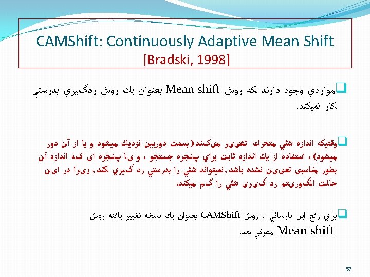
![CAMShift: Continuously Adaptive Mean Shift [Bradski, 1998] 56](https://slidetodoc.com/presentation_image_h/8aa29e03c2fac917ed9d60187a40173c/image-54.jpg "CAMShift: Continuously Adaptive Mean Shift [Bradski, 1998] 56")


- Slides: 70
Mean shift A segmentation and tracking algorithm http: //test. netii. net 1
Mean shift, the history � Mean shift was first proposed by Fukunaga and Hostetler (Fukunaga & Hostetler, 1975), � Later adapted by Cheng (Cheng, 1995) for the purpose of image analysis. � Recently it was extended by Comaniciu, Meer and Ramesh to low-level vision problems, including, segmentation (Comaniciu & Meer, 2002), adaptive smoothing (Comaniciu & Meer, 2002) and tracking (Comaniciu, Ramesh & Meer, 2003). 2
8
9
10
11
12
Mean-Shift Algorithm �Consider a set S of n data points xi (i = 1, 2, … , n) in d-Dimensional Euclidean space X. In other word xi is a d dimensional feature vector. �Let K(x) denote a kernel function that indicates how much point x contributes to the estimation of the mean. �Note that only the points located inside the moving window will contribute to calculation of mean. 13
Mean-Shift Algorithm �Let K(x) denote a kernel function that indicates how much point x contributes to the estimation of the mean. �Then, the sample mean m at x with kernel K is given by �The difference m(x) - x is called mean shift. �Note that x is the point considered to be at the center of search window. �And xi ‘s are all data points located inside the search window. 14
Mean-Shift Algorithm �Mean shift algorithm: iteratively moves a data point x (located at the center of a search window) to its mean m(x) position (that is the center of gravity of all data points located inside the search window). �In each iteration, x window center) m(x). (Now m(x) is considered as �The algorithm stops when m(x) = x. �The sequence x; m(x); m(m(x)); … is called the trajectory of x. �If sample means are computed at multiple points, then at each iteration, update is done simultaneously to all these points. 15
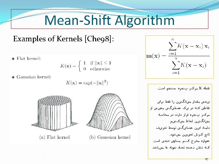
Mean-Shift Algorithm �Remember that x is a feature vector. �Typically, kernel K is a function of x) (square norm of �k is called a profile of K. �Properties of profile k is as follows: 16
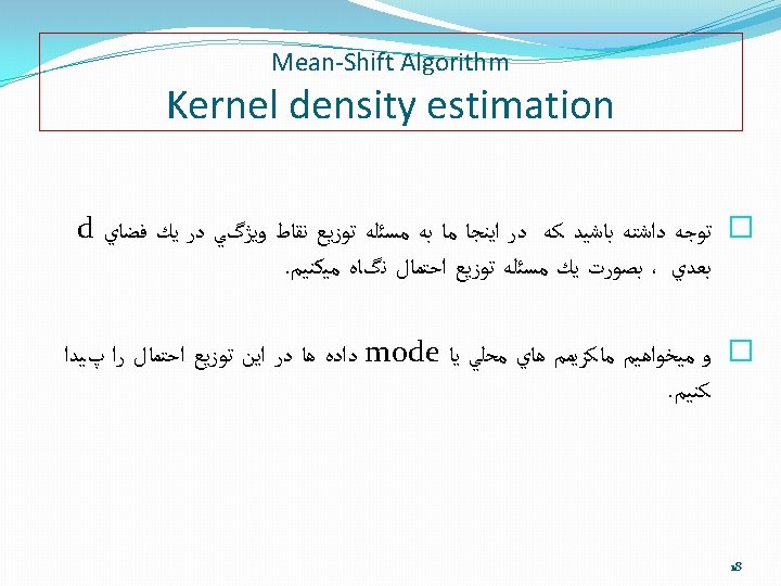
Mean-Shift Algorithm Kernel density estimation �Parzen window technique is a popular method for estimating the probability density [CRM 00, CRM 02, DH 73]. �For a set of n data points xi in d-Dimensional space, the kernel density estimate with kernel K(x) (profile k(x)) and radius h is: kernel density estimate (6) Profile of K 20
Mean-Shift Algorithm Kernel density estimation � The mean square error is minimized by the Epanechinkov kernel: . ﺭﺍ ﺣﺪ ﺍﻗﻞ ﻣﻴﻜﻨﺪ MSE � ﺑﻌﺒﺎﺭﺕ ﺩﻳگﺮ ﺍﺳﺘﻔﺎﺩﻩ ﺍﺯ ﻛﺮﻧﻞ ﻓﻮﻕ ﺧﻄﺎﻱ � where , d refers to dimensional of feature vector, Cd is the volume of the unit d-Dimensional sphere, with the following profile: 22
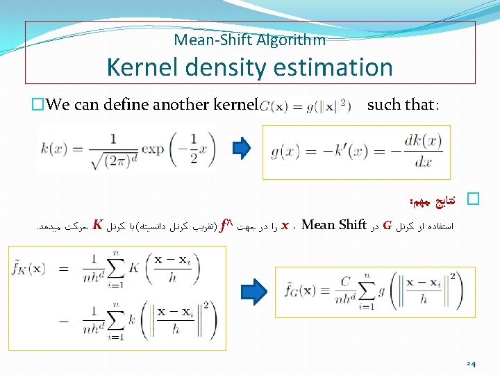
Mean-Shift Algorithm Kernel density estimation �A more commonly used kernel is Gaussian 23
Mean-Shift Algorithm Kernel density estimation � f^ : kernel density estimate. f^(G): density estimate with kernel G � Where C is a normalization constant. � h is the kernel radius � Mean shift M with kernel G is MG(x) = m(x) - x Mean shift 25
Examples for Mean shift clustering �Find features (color, gradients, texture, etc). �Initialize windows at individual feature points. �Perform mean shift for each window until convergence. �Merge windows that end up near the same “peak” or mode. 28
Examples for Mean shift clustering In this example, feature is color considered in L*u*v* color model. So, a point that is a feature vector has 3 components as L*, u* and v*. Note that each point in feature space (a) or (b) corresponds to one pixel. Meanshift calculation will be carried on for every point in feature space. A local maxima In (b) points that have converged to the same mean point are displayed with their real color in RGB color image. 29
Examples for Mean shift clustering Note how points are moving towards the local maximas (modes) that represents the center of gravity for those data points. In this example we have ended up with 7 segments (modes). A local maxima 30
Examples for Mean shift clustering Original Result of Mean-shift Segmentation. All points in image that their corresponding point in feature space have converged to the same mean point are given the RGB color of that mean point. (L*u*v* value of the mean point is converted to RGB) 31
Mean shift: The Cons and Pros: �Does not assume spherical clusters. �Just a single parameter (window size). �Finds variable number of modes (clusters), depending on the given data. �Robust to outliers. Cons: �Output depends on window size. �Computationally expensive (calculation must be carried out for all points in the feature space). �Does not scale well with dimension of feature space. 32
Mean Shift Tracking 33
Main steps in Mean shift tracking algorithm 45
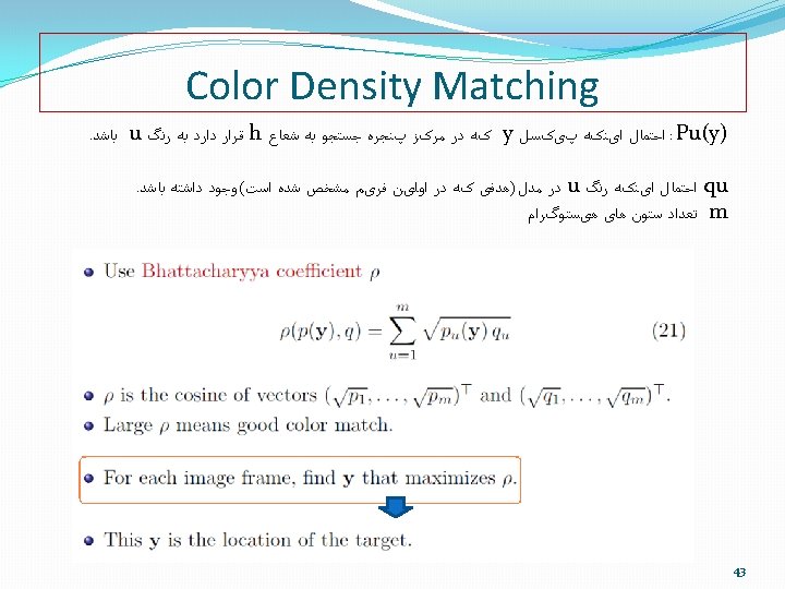
Main steps in Mean shift tracking algorithm � qu is the probability that color u exists in model. � Given {qu} of model and location y’ of target in previous frame: 1. 2. 3. Initialize location of target in current frame as y. // y is the center of a search window Compute {pu(y)} and ρ(p(y), q). Apply mean shift: Compute z, as a new center for window, for the window centered at y and the data points yi inside that window: ( z is the mean or centeriod of all points yi inside the window ) g is the profile of a kernel G 46
Main steps in Mean shift tracking algorithm 4. Compute {pu(z)} and ρ(p(z) , q) 5. While ( ρ(p(z) , q) < ρ(p(y) , q) ) do z ½(y+z) 6. If || z - y || is small enough, then stop Else y z goto (1) 47
Detail description of steps in mean shift tracking algorithm. 3. Apply mean shift: that is to compute new location for y as This new location, z, is found among data points yi that are located in a window with radius h centered in y Note that z will be the widow center in the new search window. 48
Mean Shift Tracking 4. Compute {pu(z)} and ρ(p(z) , q). 5. While ρ(p(z) , q) < ρ(p(y) , q), do z ½(y+z). 6. If || z-y || is small enough, then stop. else, set y z, and goto (1). � Step 5 is used to validate the target's new location. � Step 5 can be stopped if y and z round off to the same pixel. � Tests show that Step 5 is needed only 0. 1% of the time. 49
Mean Shift Tracking 4. Compute {pu(z)} and ρ(p(z) , q). 5. While ρ(p(z) , q) < ρ(p(y) , q), do z ½(y+z). 6. If || z-y || is small enough, then stop. else, set y z, and goto (1). � Step 6: can stop the algorithm if y and z round off to the same pixel. 50
Mean Shift Tracking To track object that changes its size and shape during time, we shall vary radius h, (the size of search window). (see [CRM 00] for details). 51
Mean Shift Tracking Frame 2 (target found) Frame 1 (Model) 52
Mean Shift Tracking Model, specified manually 53
Mean Shift References 54
Tracking References 55
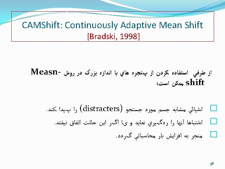
CAMShift: Continuously Adaptive Mean Shift [Bradski, 1998] 56
Mean Shift Tracking Target. Model Since we know That the object is moving toward us, we can enlarge the search window Size. Model Target 67
70
Tracking before radars 71
72
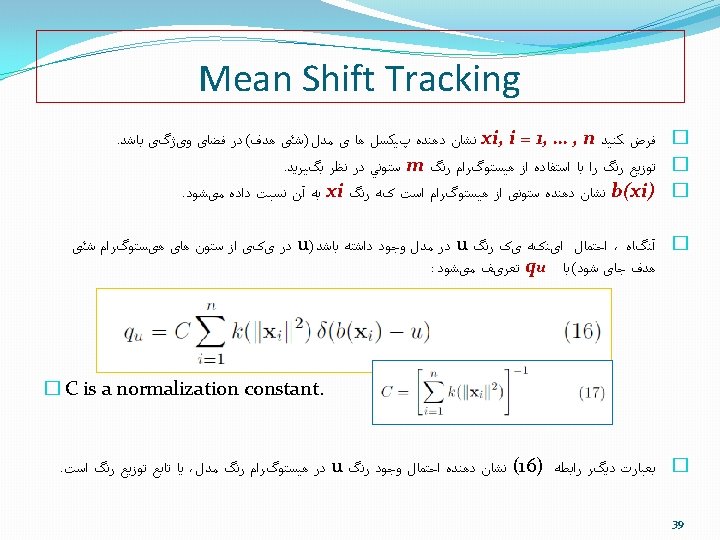
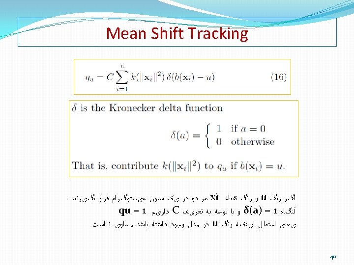
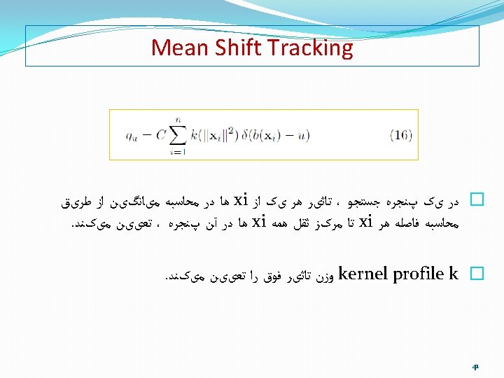
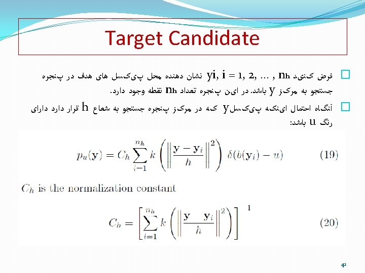
Mean Shift Tracking �Let xi, i = 1, … , n, denote pixel locations of model centered at 0. �Represent color distribution by discrete m-bin color histogram. �Let b(xi) denote the color bin of the color at xi. �Assume size of model is normalized; so, kernel radius h = 1. �Then, the probability q of color u in the model is �C is a normalization constant. 73