ME 431 System Dynamics Dept of Mechanical Engineering

ME 431 System Dynamics Dept of Mechanical Engineering

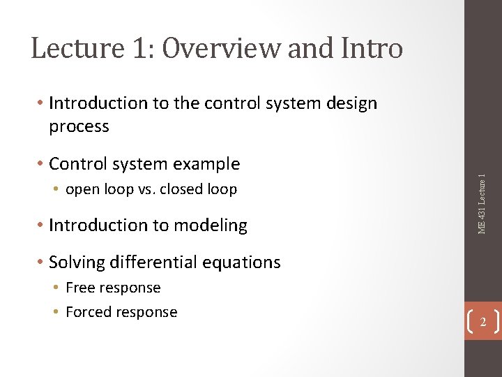
Lecture 1: Overview and Intro • Control system example • open loop vs. closed loop • Introduction to modeling ME 431 Lecture 1 • Introduction to the control system design process • Solving differential equations • Free response • Forced response 2

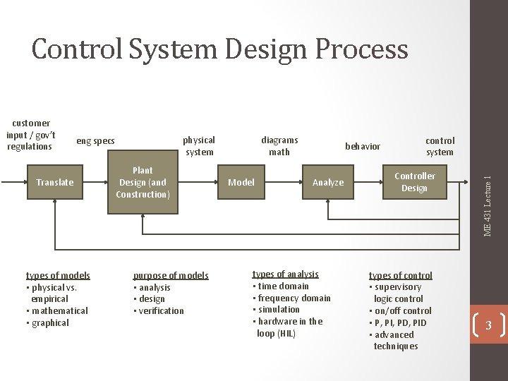
Control System Design Process physical system eng specs Translate types of models • physical vs. empirical • mathematical • graphical Plant Design (and Construction) purpose of models • analysis • design • verification diagrams math Model behavior Analyze types of analysis • time domain • frequency domain • simulation • hardware in the loop (HIL) control system Controller Design types of control • supervisory logic control • on/off control • P, PI, PD, PID • advanced techniques ME 431 Lecture 1 customer input / gov’t regulations 3

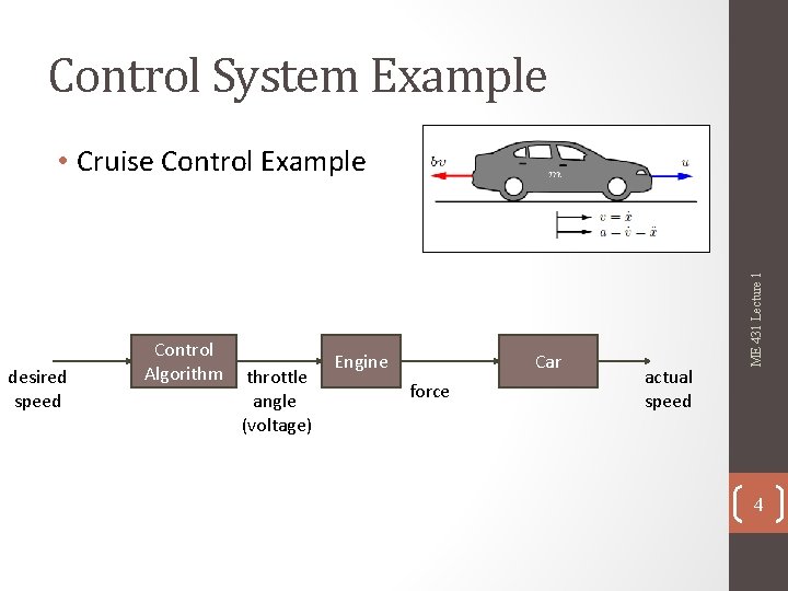
Control System Example desired speed Control Algorithm throttle angle (voltage) Engine Car force actual speed ME 431 Lecture 1 • Cruise Control Example 4

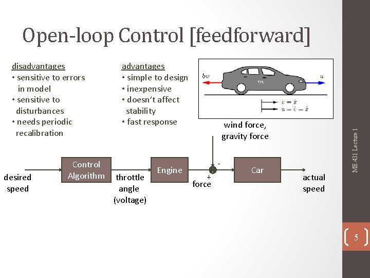
disadvantages • sensitive to errors in model • sensitive to disturbances • needs periodic recalibration desired speed Control Algorithm advantages • simple to design • inexpensive • doesn’t affect stability • fast response throttle angle (voltage) Engine wind force, gravity force + force Car actual speed ME 431 Lecture 1 Open-loop Control [feedforward] 5

Closed-loop Control [feedback] R desired speed + E - advantages • robust to errors in model • robust to disturbances D wind force, gravity force CONTROLLER ACTUATOR PLANT -U Control Engine Car Algorithm throttle + force angle (voltage) SENSOR measured speed Y actual speed ME 431 Lecture 1 disadvantages • extra complexity • extra cost • can affect stability • can be slow to respond Speedometer 6

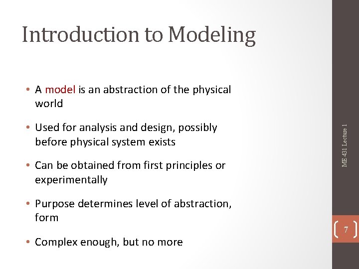
Introduction to Modeling • Used for analysis and design, possibly before physical system exists • Can be obtained from first principles or experimentally ME 431 Lecture 1 • A model is an abstraction of the physical world • Purpose determines level of abstraction, form • Complex enough, but no more 7

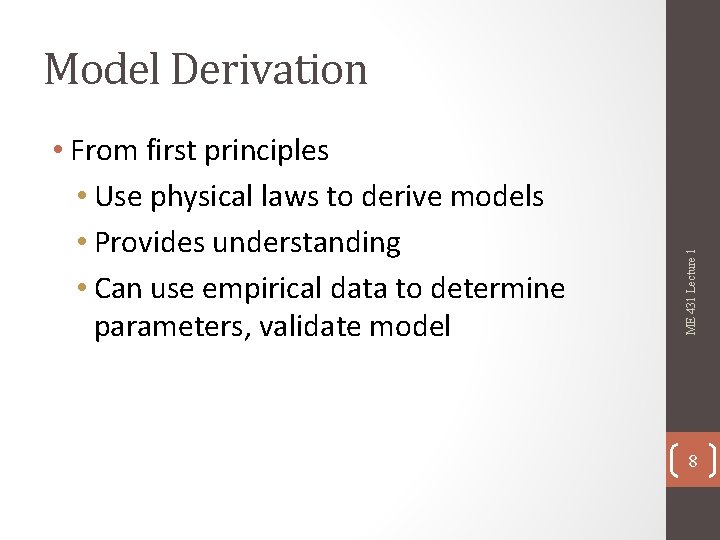
• From first principles • Use physical laws to derive models • Provides understanding • Can use empirical data to determine parameters, validate model ME 431 Lecture 1 Model Derivation 8

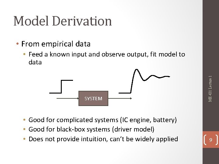
Model Derivation • From empirical data SYSTEM • Good for complicated systems (IC engine, battery) • Good for black-box systems (driver model) • Does not provide intuition, can’t be widely applied ME 431 Lecture 1 • Feed a known input and observe output, fit model to data 9

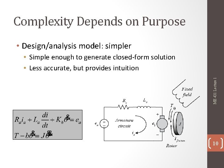
Complexity Depends on Purpose • Design/analysis model: simpler ME 431 Lecture 1 • Simple enough to generate closed-form solution • Less accurate, but provides intuition 10

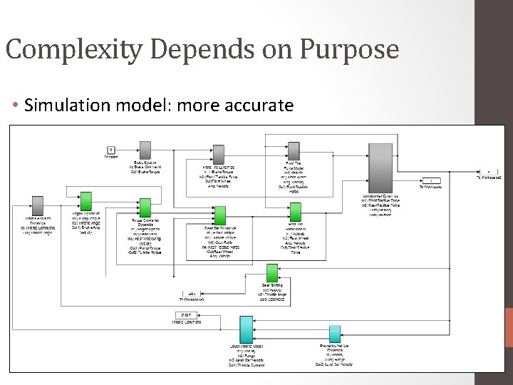
Complexity Depends on Purpose • Simulation model: more accurate

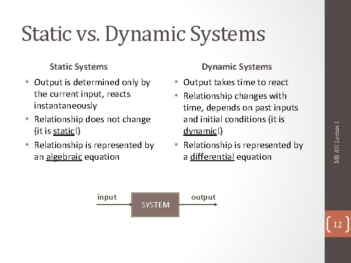
Static vs. Dynamic Systems • Output is determined only by the current input, reacts instantaneously • Relationship does not change (it is static!) • Relationship is represented by an algebraic equation input SYSTEM • Output takes time to react • Relationship changes with time, depends on past inputs and initial conditions (it is dynamic!) • Relationship is represented by a differential equation ME 431 Lecture 1 Static Systems output 12

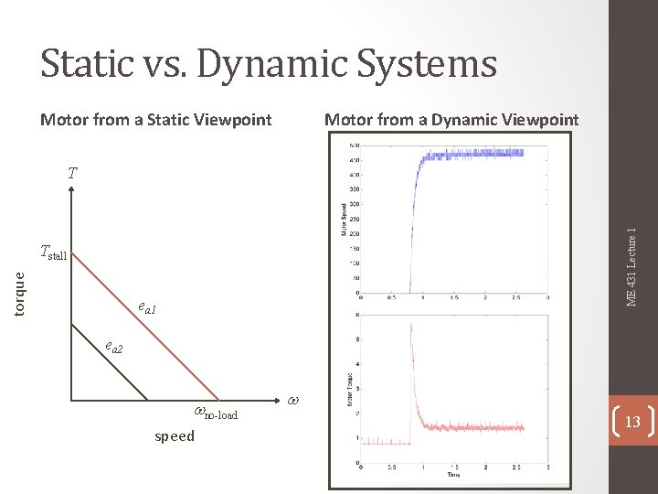
Static vs. Dynamic Systems Motor from a Static Viewpoint Motor from a Dynamic Viewpoint ME 431 Lecture 1 T torque Tstall ea 1 ea 2 wno-load speed w 13

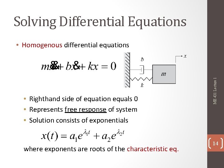
Solving Differential Equations • Righthand side of equation equals 0 • Represents free response of system • Solution consists of exponentials where exponents are roots of the characteristic eq. ME 431 Lecture 1 • Homogenous differential equations 14

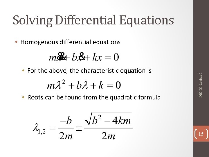
Solving Differential Equations • For the above, the characteristic equation is • Roots can be found from the quadratic formula ME 431 Lecture 1 • Homogenous differential equations 15

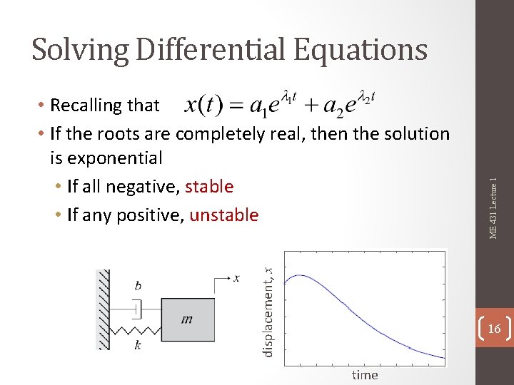
displacement, x • Recalling that • If the roots are completely real, then the solution is exponential • If all negative, stable • If any positive, unstable ME 431 Lecture 1 Solving Differential Equations 16 time

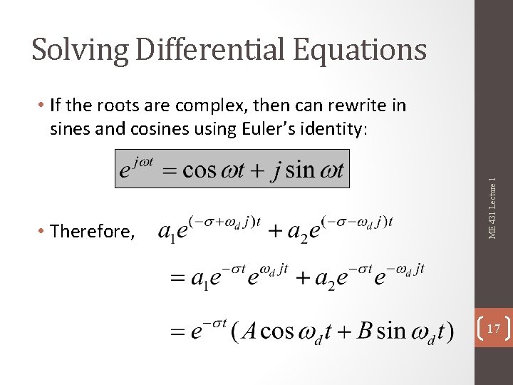
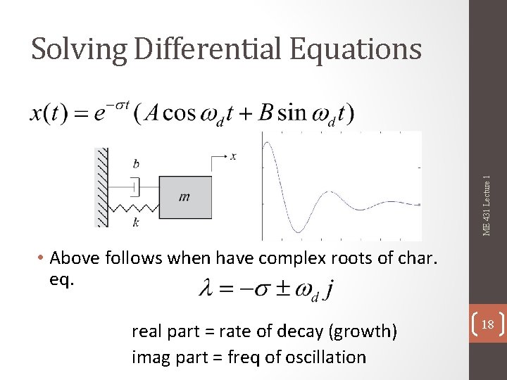
Solving Differential Equations • Therefore, ME 431 Lecture 1 • If the roots are complex, then can rewrite in sines and cosines using Euler’s identity: 17

ME 431 Lecture 1 Solving Differential Equations • Above follows when have complex roots of char. eq. real part = rate of decay (growth) imag part = freq of oscillation 18

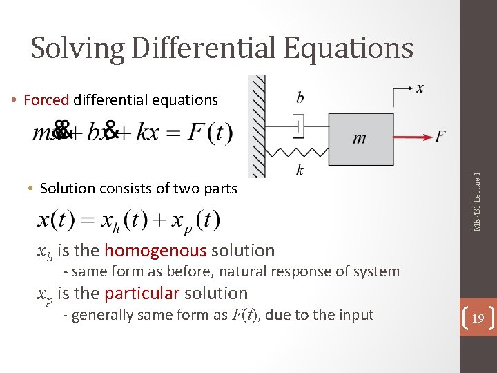
Solving Differential Equations • Solution consists of two parts ME 431 Lecture 1 • Forced differential equations xh is the homogenous solution - same form as before, natural response of system xp is the particular solution - generally same form as F(t), due to the input 19

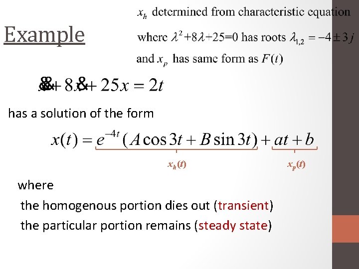
Example has a solution of the form xh(t) where the homogenous portion dies out (transient) the particular portion remains (steady state) xp(t)

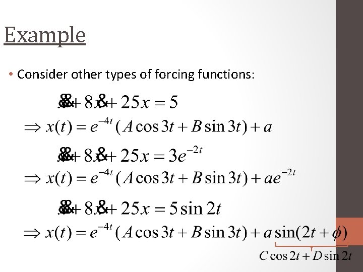
Example • Consider other types of forcing functions:

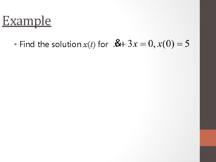
Example • Find the solution x(t) for

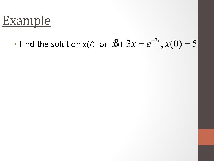
Example • Find the solution x(t) for

Example (continued)