MDPs cont Reinforcement Learning Tamara Berg CS 560
 & Reinforcement Learning Tamara Berg CS 560 Artificial Intelligence Many slides throughout")
MDPs (cont) & Reinforcement Learning Tamara Berg CS 560 Artificial Intelligence Many slides throughout the course adapted from Svetlana Lazebnik, Dan Klein, Stuart Russell, Andrew Moore, Percy Liang, Luke Zettlemoyer

Announcements • HW 2 online: CSPs and Games – Due Oct 8, 11: 59 pm (start now!) • Mid-term exam next Wed, Sept 30 – – Held during regular class time. Closed book. You may bring a calculator. Written questions (no coding). Ric will lead an in class mid-term review/exercises session in class on Sept 28.
 Intro to AI, agents and environments Turing test Rationality Expected utility")
Exam topics 1) Intro to AI, agents and environments Turing test Rationality Expected utility maximization PEAS Environment characteristics: fully vs. partially observable, deterministic vs. stochastic, episodic vs. sequential, static vs. dynamic, discrete vs. continuous, single-agent vs. multiagent, known vs. unknown 2) Search problem formulation: initial state, actions, transition model, goal state, path cost State space graph Search tree Frontier, Explored set Evaluation of search strategies: completeness, optimality, time complexity, space complexity Uninformed search strategies: breadth-first search, uniform cost search, depth-first search, iterative deepening search Informed search strategies: greedy best-first, A*, weighted A* Heuristics: admissibility, dominance
 Constraint satisfaction problems Backtracking search Heuristics: most constrained/most constraining variable, least")
Exam topics 3) Constraint satisfaction problems Backtracking search Heuristics: most constrained/most constraining variable, least constraining value Forward checking, constraint propagation, arc consistency Taking advantage of structure – connected components, Tree-structured CSPs Local search Formulating photo ordering as a CSP 4) Games Zero-sum games Game tree Minimax/Expectiminimax search Alpha-beta pruning Evaluation function Quiescence search Horizon effect Stochastic elements in games
 Markov decision processes Markov assumption, transition model, policy Bellman equation Value")
Exam topics 5) Markov decision processes Markov assumption, transition model, policy Bellman equation Value iteration Policy iteration 6) Reinforcement learning Model-based vs. model-free approaches Passive vs Active Exploration vs. exploitation Direct Estimation TD Learning TD Q-learning Applications to backgammon, quadruped locomotion, helicopter flying

Markov Decision Processes Stochastic, sequential environments Image credit: P. Abbeel and D. Klein

Markov Decision Processes • Components: – States s, beginning with initial state s 0 – Actions a • Each state s has actions A(s) available from it – Transition model P(s’ | s, a) • Markov assumption: the probability of going to s’ from s depends only on s and a and not on any other past actions or states – Reward function R(s) • Policy (s): the action that an agent takes in any given state – The “solution” to an MDP

Overview • First, we will look at how to “solve” MDPs, ie find the optimal policy when the transition model and the reward function are known • Second, we will consider reinforcement learning, where we don’t know the rules of the environment or the consequences of our actions
 = -0. 04")
Grid world Transition model: 0. 1 0. 8 0. 1 R(s) = -0. 04 for every non-terminal state Source: P. Abbeel and D. Klein

Goal: Policy Source: P. Abbeel and D. Klein
 = -0. 04 for every non-terminal state")
Grid world Optimal policy when R(s) = -0. 04 for every non-terminal state
:")
Grid world • Optimal policies for other values of R(s):

Solving MDPs • MDP components: – States s – Actions a – Transition model P(s’ | s, a) – Reward function R(s) • The solution: – Policy (s): mapping from states to actions – How to find the optimal policy?
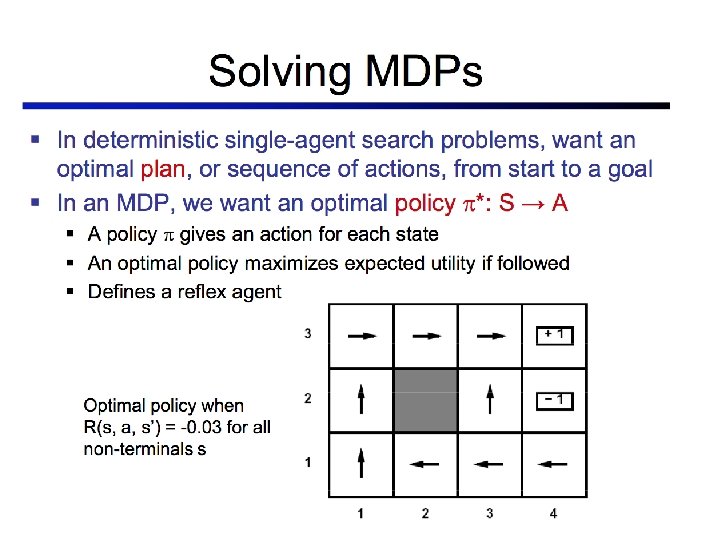

Maximizing expected utility • The optimal policy should maximize the expected utility over all possible state sequences produced by following that policy: • How to define the utility of a state sequence? – Sum of rewards of individual states – Problem: infinite state sequences

Utilities of state sequences • Normally, we would define the utility of a state sequence as the sum of the rewards of the individual states • Problem: infinite state sequences • Solution: discount the individual state rewards by a factor between 0 and 1: – Sooner rewards count more than later rewards – Makes sure the total utility stays bounded – Helps algorithms converge

Utilities of states • Expected utility obtained by policy starting in state s: • The “true” utility (value) of a state, is the expected sum of discounted rewards if the agent executes an optimal policy starting in state s

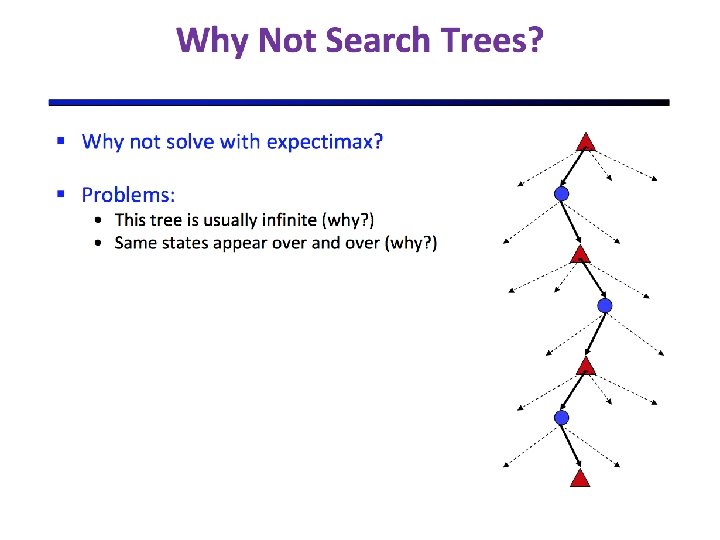
Finding the utilities of states • What is the expected utility of taking action a in state s? Max node Chance node P(s’ | s, a) • How do we choose the optimal action? U(s’) • What is the recursive expression for U(s) in terms of the utilities of its successor states?

The Bellman equation • Recursive relationship between the utilities of successive states: Receive reward R(s) Choose optimal action a End up here with P(s’ | s, a) Get utility U(s’) (discounted by )

The Bellman equation • Recursive relationship between the utilities of successive states: • For N states, we get N equations in N unknowns – Solving them solves the MDP – Two methods: value iteration and policy iteration
 = 0 • Iterate")
Method 1: Value iteration • Start out with every U(s) = 0 • Iterate until convergence – During the ith iteration, update the utility of all states (simultaneously) according to this rule: • In the limit of infinitely many iterations, guaranteed to find the correct utility values – In practice, don’t need an infinite number of iterations…
= -0. 25 for")
Value iteration • Run value iteration on the following grid-world: R(s)= -0. 25 for all non-terminal states Transition model: 0. 7 chance of going in desired direction, 0. 1 chance of going in any of the other 3 directions. If agent moves into a wall, it stays put.
= -0. 25")
Value iteration • Run value iteration on the following grid-world: 0 R(s)= -0. 25 for all non-terminal states 0 0 0 0 Transition model: 0. 7 chance of going in desired direction, 0. 1 chance of going in any of the other 3 directions. If agent moves into a wall, it stays put.

Value iteration demo
- Slides: 25