MCMC for Stochastic Epidemic Models Philip D ONeill

MCMC for Stochastic Epidemic Models Philip D. O’Neill School of Mathematical Sciences University of Nottingham

This includes joint work with… Tom Britton (Stockholm) n Niels Becker (ANU, Canberra) n Gareth Roberts (Lancaster) n Peter Marks (NHS, Derbyshire PCT) n

Contents 1. MCMC: overview and basics n 2. Example: Vaccine efficacy n 3. Data augmentation n 4. Example: SIR epidemic model n 5. Model choice n 6. Example: Norovirus outbreak n 7. Other topics n

1. Markov chain Monte Carlo (MCMC) Overview and basics The key problem is to explore a density function π known up to proportionality. n The output of an MCMC algorithm is a sequence of samples from the correctly normalised π. n These samples can be used to estimate summaries of π, e. g. its mean, variance. n

How MCMC works Key idea is to construct a discrete time Markov chain X 1, X 2, X 3, … on state space S whose stationary distribution is π. n If P(dy, dx) is the transitional kernel of the chain this means that n

How MCMC works (2) n Subject to some technical conditions, Distribution of Xn → π as n → n Thus to obtain samples from π we simulate the chain and sample from it after a “long time”.

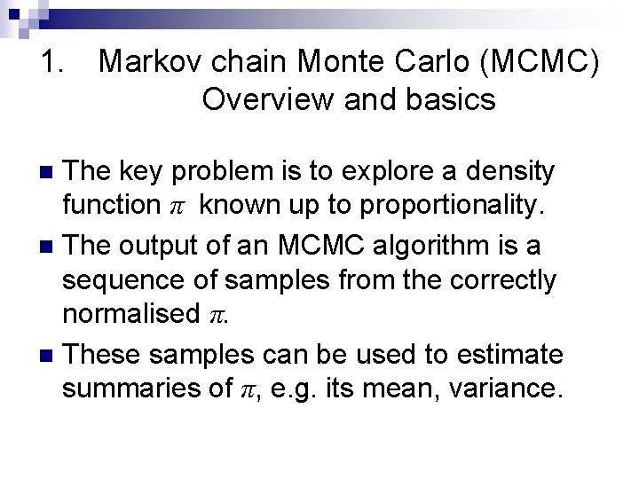
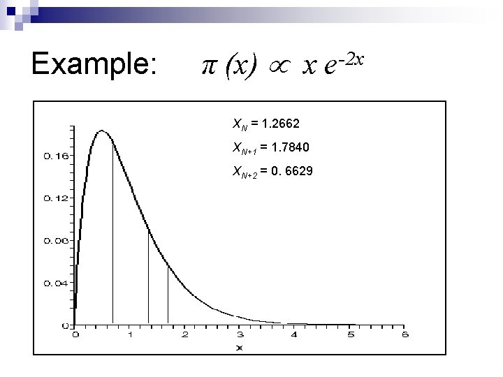
Example: π (x) x e-2 x

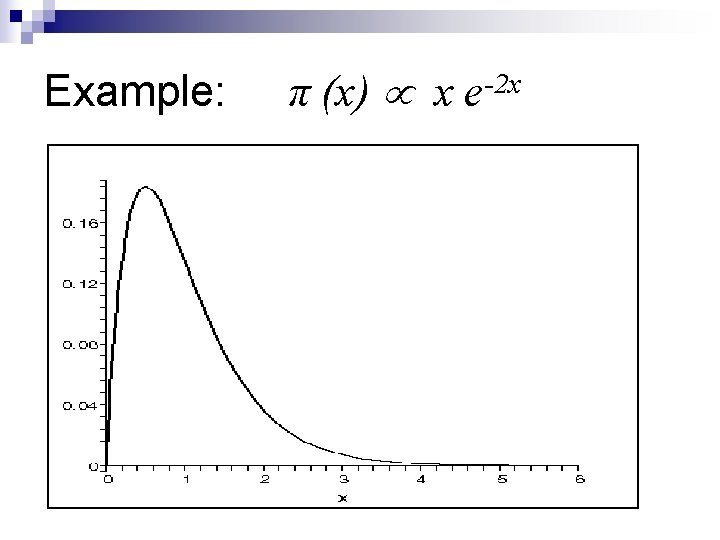
Example: X 1, X 2, … π (x) x e-2 x XN = 1. 2662

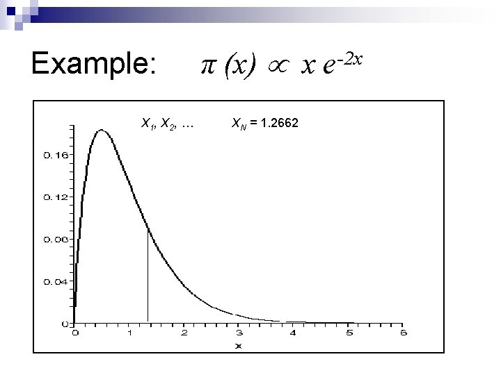
Example: π (x) x e-2 x XN = 1. 2662 XN+1 = 1. 7840

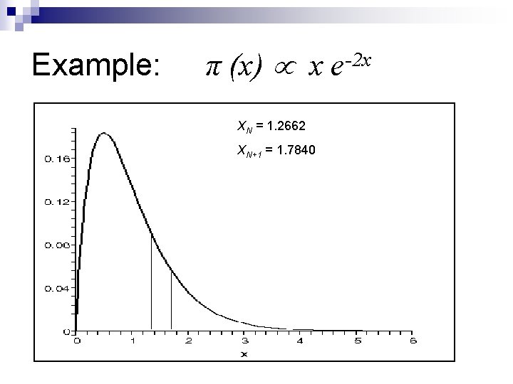
Example: π (x) x e-2 x XN = 1. 2662 XN+1 = 1. 7840 XN+2 = 0. 6629

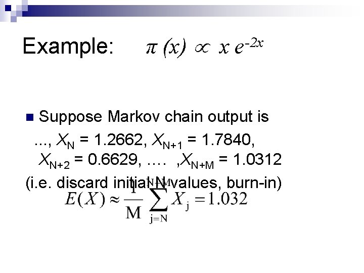
Example: π (x) x e-2 x Suppose Markov chain output is. . . , XN = 1. 2662, XN+1 = 1. 7840, XN+2 = 0. 6629, …. , XN+M = 1. 0312 (i. e. discard initial N values, burn-in) n

How to build the Markov chain Surprisingly, there are many ways to construct a Markov chain with stationary distribution π. n Perhaps the simplest is the Metropolis. Hastings algorithm. n

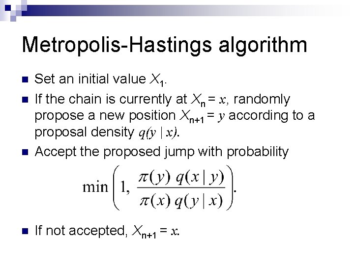
Metropolis-Hastings algorithm n Set an initial value X 1. If the chain is currently at Xn = x, randomly propose a new position Xn+1 = y according to a proposal density q(y | x). Accept the proposed jump with probability n If not accepted, Xn+1 = x. n n

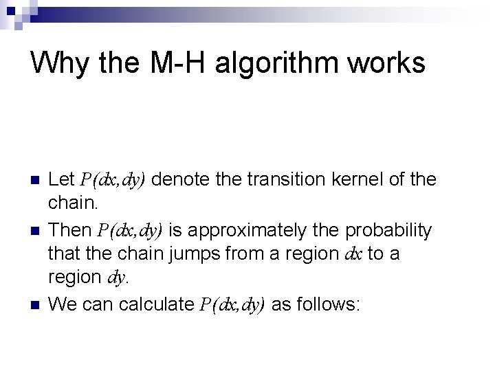
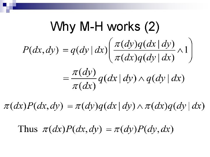
Why the M-H algorithm works n n n Let P(dx, dy) denote the transition kernel of the chain. Then P(dx, dy) is approximately the probability that the chain jumps from a region dx to a region dy. We can calculate P(dx, dy) as follows:

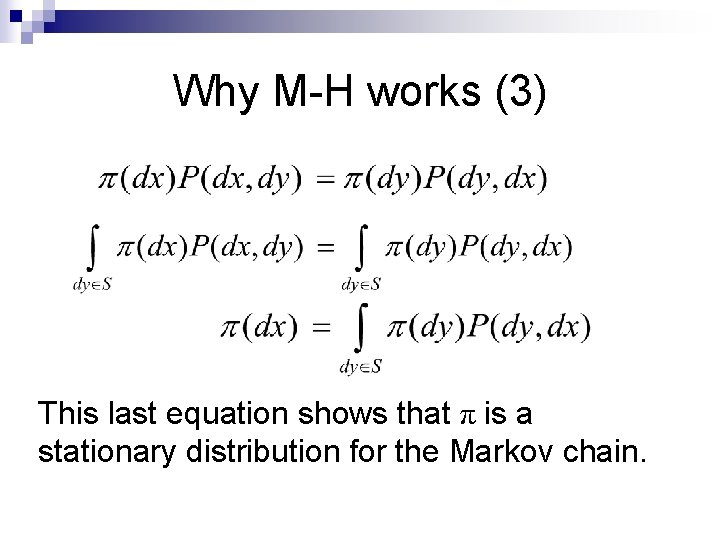
Why M-H works (2)

Why M-H works (3) This last equation shows that π is a stationary distribution for the Markov chain.

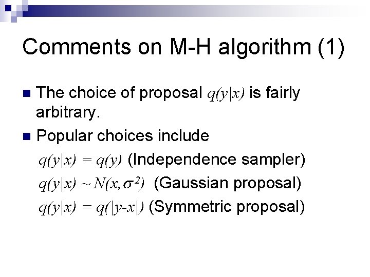
Comments on M-H algorithm (1) The choice of proposal q(y|x) is fairly arbitrary. n Popular choices include q(y|x) = q(y) (Independence sampler) q(y|x) ~ N(x, 2) (Gaussian proposal) q(y|x) = q(|y-x|) (Symmetric proposal) n

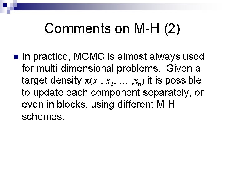
Comments on M-H (2) n In practice, MCMC is almost always used for multi-dimensional problems. Given a target density π(x 1, x 2, … , xn) it is possible to update each component separately, or even in blocks, using different M-H schemes.

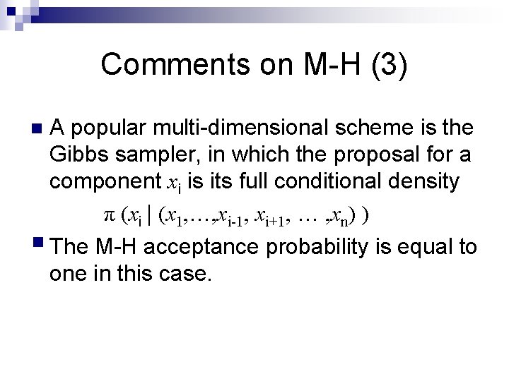
Comments on M-H (3) A popular multi-dimensional scheme is the Gibbs sampler, in which the proposal for a component xi is its full conditional density π (xi | (x 1, …, xi-1, xi+1, … , xn) ) § The M-H acceptance probability is equal to one in this case. n

General comments on MCMC How to check convergence? There is no guaranteed way. Visual inspection of trace plots; diagnostic tools (e. g. looking at autocorrelation). n Starting values – try a range n Acceptance rates – not too large/small n Mixing – how fast does the chain move around? n

Contents 1. MCMC: overview and basics n 2. Example: Vaccine efficacy n 3. Data augmentation n 4. Example: SIR epidemic model n 5. Model choice n 6. Example: Norovirus outbreak n 7. Other topics n

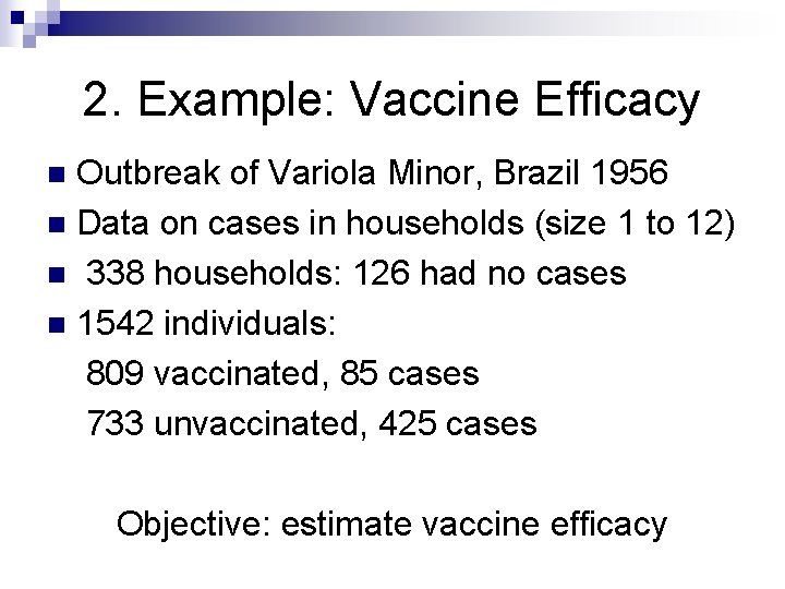
2. Example: Vaccine Efficacy Outbreak of Variola Minor, Brazil 1956 n Data on cases in households (size 1 to 12) n 338 households: 126 had no cases n 1542 individuals: 809 vaccinated, 85 cases 733 unvaccinated, 425 cases n Objective: estimate vaccine efficacy

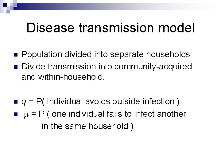
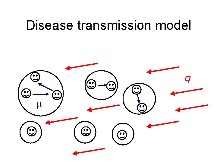
Disease transmission model n n Population divided into separate households. Divide transmission into community-acquired and within-household. q = P( individual avoids outside infection ) = P ( one individual fails to infect another in the same household )

Disease transmission model q

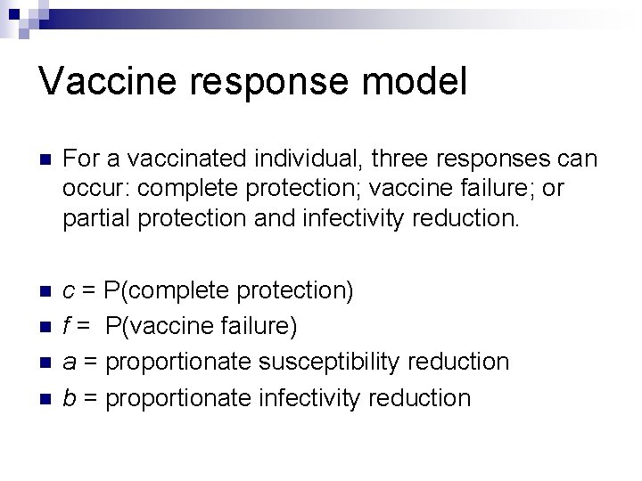
Vaccine response model n For a vaccinated individual, three responses can occur: complete protection; vaccine failure; or partial protection and infectivity reduction. n c = P(complete protection) f = P(vaccine failure) a = proportionate susceptibility reduction b = proportionate infectivity reduction n

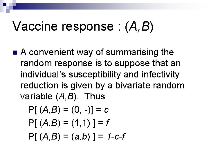
Vaccine response : (A, B) n A convenient way of summarising the random response is to suppose that an individual’s susceptibility and infectivity reduction is given by a bivariate random variable (A, B). Thus P[ (A, B) = (0, -)] = c P[ (A, B) = (1, 1) ] = f P[ (A, B) = (a, b) ] = 1 -c-f

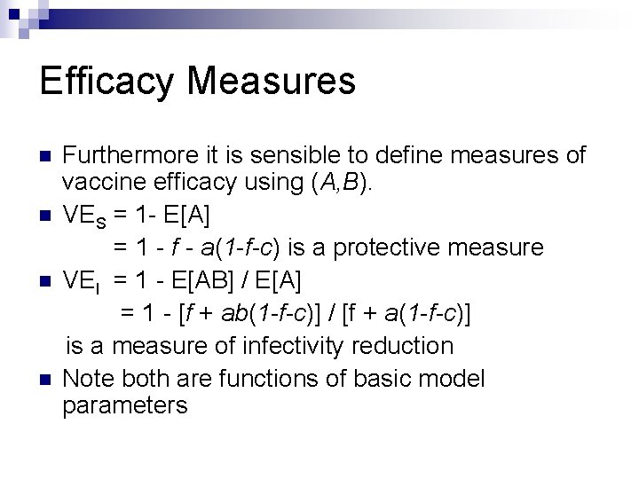
Efficacy Measures n n Furthermore it is sensible to define measures of vaccine efficacy using (A, B). VES = 1 - E[A] = 1 - f - a(1 -f-c) is a protective measure VEI = 1 - E[AB] / E[A] = 1 - [f + ab(1 -f-c)] / [f + a(1 -f-c)] is a measure of infectivity reduction Note both are functions of basic model parameters

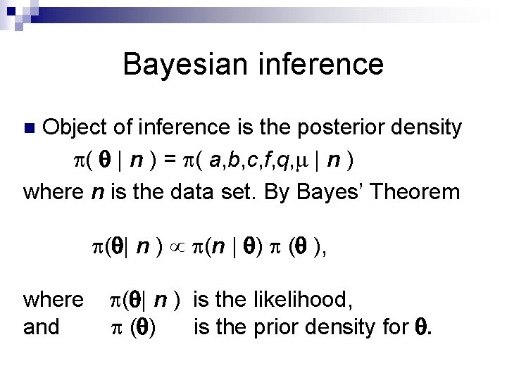
Bayesian inference Object of inference is the posterior density ( | n ) = ( a, b, c, f, q, | n ) where n is the data set. By Bayes’ Theorem n ( | n ) (n | ) ( ), where and ( | n ) is the likelihood, ( ) is the prior density for .

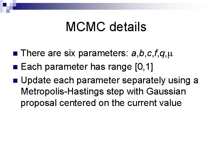
MCMC details There are six parameters: a, b, c, f, q, n Each parameter has range [0, 1] n Update each parameter separately using a Metropolis-Hastings step with Gaussian proposal centered on the current value n

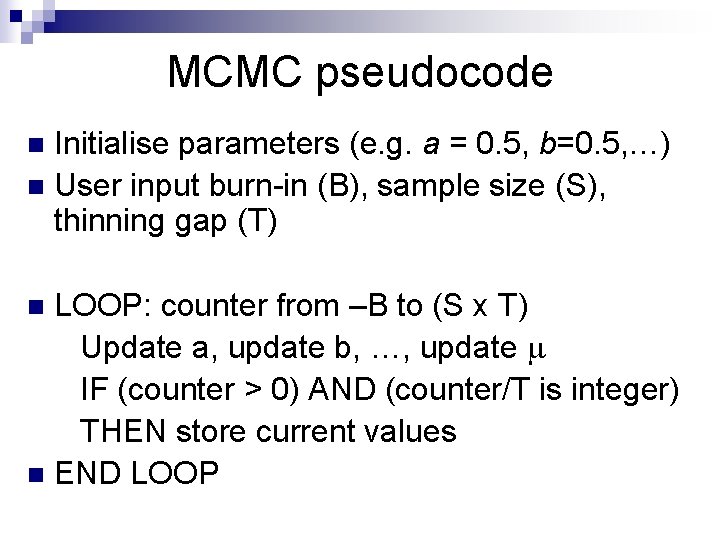
MCMC pseudocode Initialise parameters (e. g. a = 0. 5, b=0. 5, …) n User input burn-in (B), sample size (S), thinning gap (T) n LOOP: counter from –B to (S x T) Update a, update b, …, update IF (counter > 0) AND (counter/T is integer) THEN store current values n END LOOP n

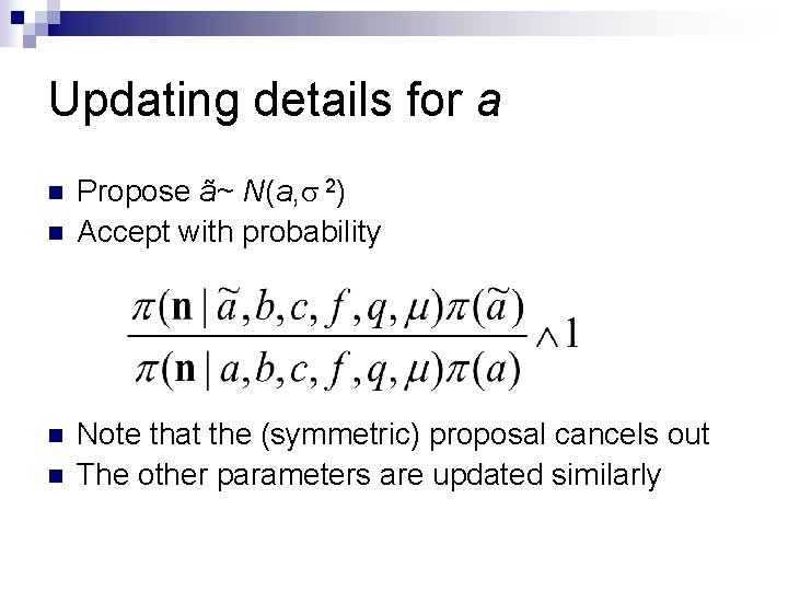
Updating details for a n n Propose ã~ N(a, 2) Accept with probability Note that the (symmetric) proposal cancels out The other parameters are updated similarly

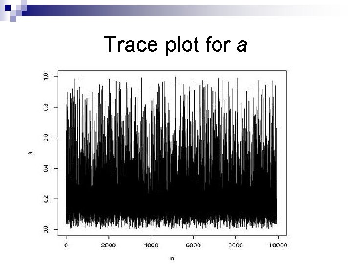
Trace plot for a

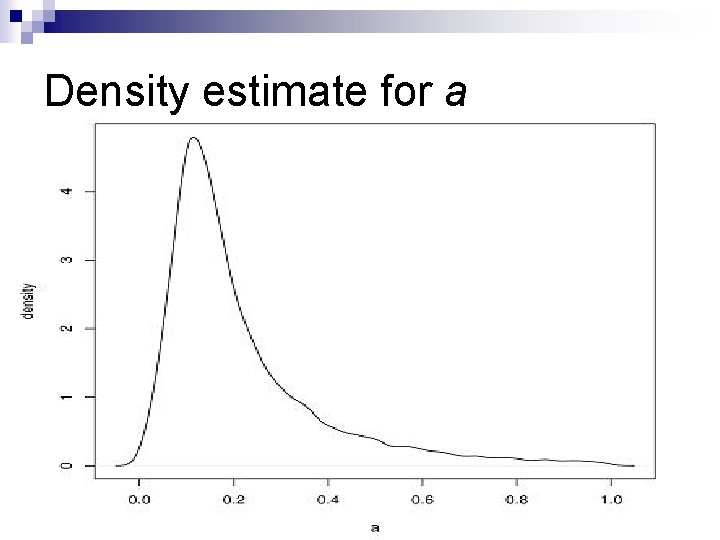
Density estimate for a

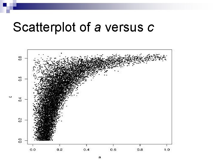
Scatterplot of a versus c

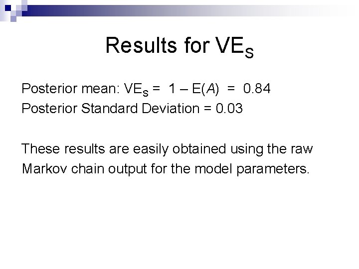
Results for VES Posterior mean: VES = 1 – E(A) = 0. 84 Posterior Standard Deviation = 0. 03 These results are easily obtained using the raw Markov chain output for the model parameters.

Contents 1. MCMC: overview and basics n 2. Example: Vaccine efficacy n 3. Data augmentation n 4. Example: SIR epidemic model n 5. Model choice n 6. Example: Norovirus outbreak n 7. Other topics n

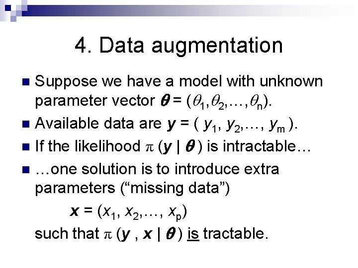
4. Data augmentation Suppose we have a model with unknown parameter vector = ( 1, 2, …, n). n Available data are y = ( y 1, y 2, …, ym ). n If the likelihood π (y | ) is intractable… n …one solution is to introduce extra parameters (“missing data”) x = (x 1, x 2, …, xp) such that π (y , x | ) is tractable. n

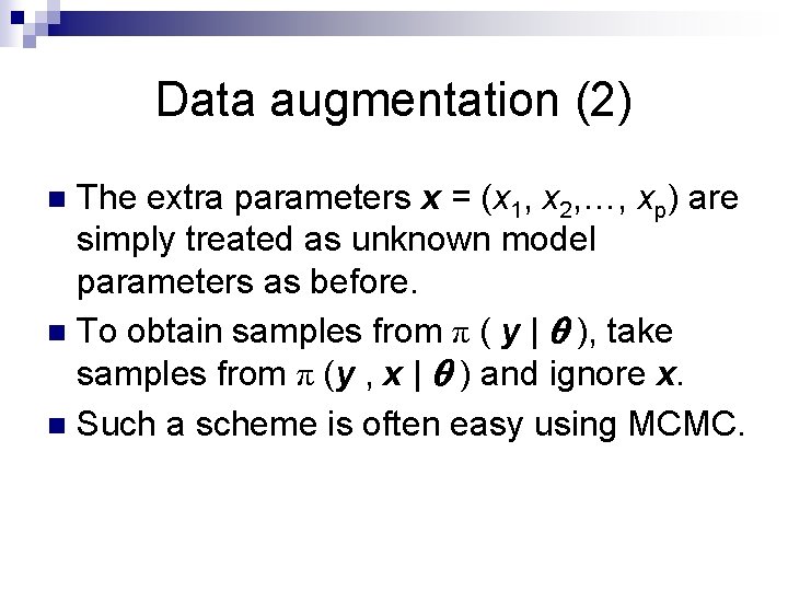
Data augmentation (2) The extra parameters x = (x 1, x 2, …, xp) are simply treated as unknown model parameters as before. n To obtain samples from π ( y | ), take samples from π (y , x | ) and ignore x. n Such a scheme is often easy using MCMC. n

Data augmentation (3) Can also add parameters to improve the mixing of the Markov chain (auxiliary variables). n Choosing how to augment data is not always obvious! n

Contents 1. MCMC: overview and basics n 2. Example: Vaccine efficacy n 3. Data augmentation n 4. Example: SIR epidemic model n 5. Model choice n 6. Example: Norovirus outbreak n 7. Other topics n

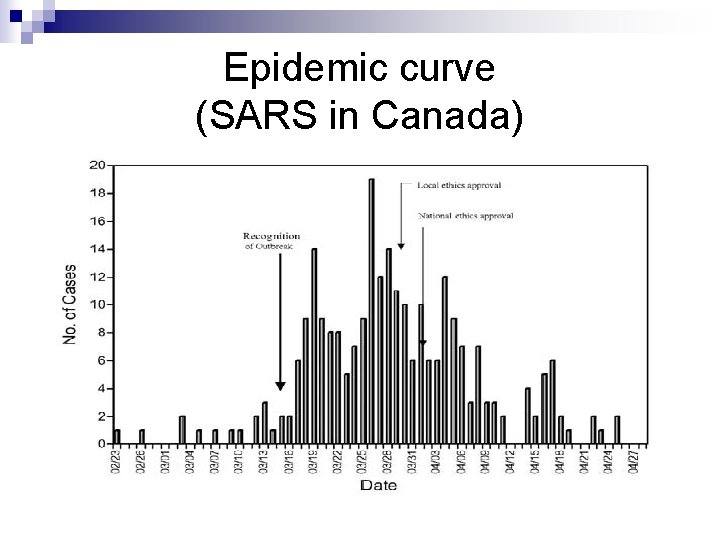
4. SIR Epidemic Model Suppose we observe daily numbers of cases during an epidemic outbreak in some fixed population. n Objective is to say something about infection rates and infectious period duration of the disease. n

Epidemic curve (SARS in Canada)

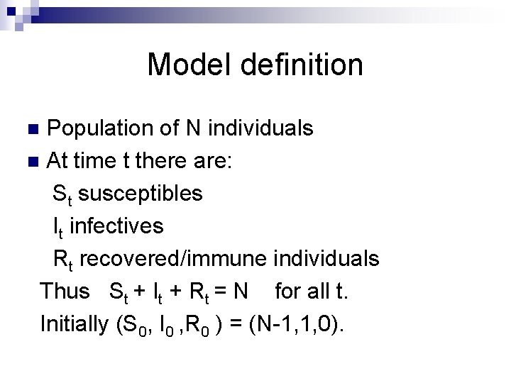
Model definition Population of N individuals n At time t there are: St susceptibles It infectives Rt recovered/immune individuals Thus St + It + Rt = N for all t. Initially (S 0, I 0 , R 0 ) = (N-1, 1, 0). n

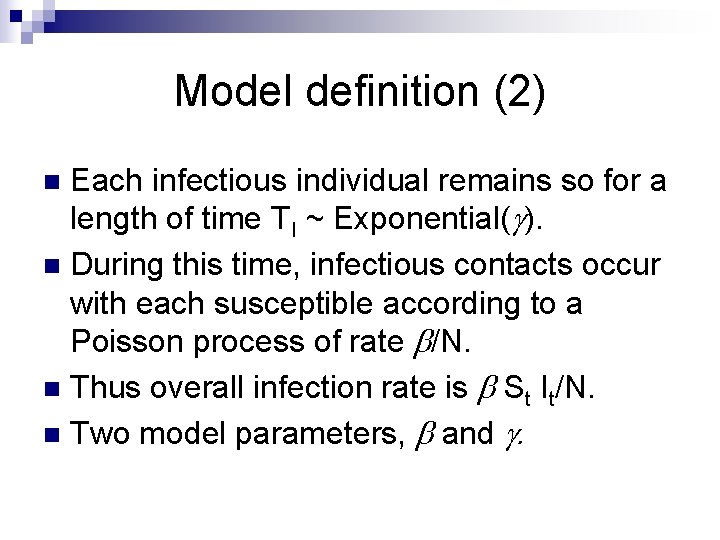
Model definition (2) Each infectious individual remains so for a length of time TI ~ Exponential( ). n During this time, infectious contacts occur with each susceptible according to a Poisson process of rate /N. n Thus overall infection rate is St It/N. n Two model parameters, and . n

Data, likelihood, augmentation Suppose we observe removals at times 0 ≤ r 1 ≤ r 2 ≤ … ≤ rn ≤ . n Define r = ( r 1, r 2 , …, rn ). n The likelihood of the data, π (r | , ), is practically intractable. n However, given the (unknown) infection times i = ( i 1, i 2 , …, in ), π (i , r | , ) is tractable. n

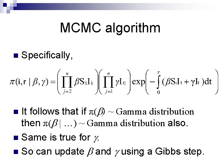
MCMC algorithm n Specifically, It follows that if π( ) ~ Gamma distribution then π( | …) ~ Gamma distribution also. n Same is true for . n So can update and using a Gibbs step. n

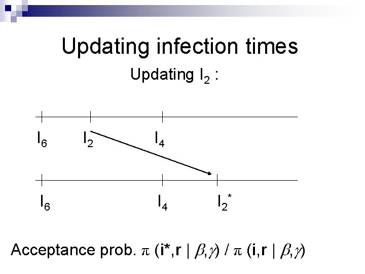
MCMC algorithm – infection times It remains to update the infection times i = ( i 1, i 2 , …, in ) n Various ways of doing this. n A simple way is to use a M-H scheme to randomly move the times. n For example, propose a new ik by picking a new time uniformly at random in (0, ). n

Updating infection times Updating I 2 : I 6 I 2 I 4 I 2* Acceptance prob. π (i*, r | , ) / π (i, r | , )

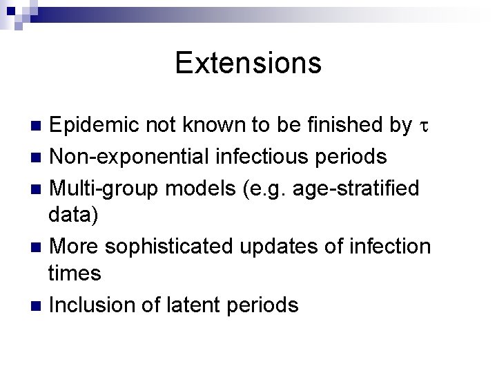
Extensions Epidemic not known to be finished by n Non-exponential infectious periods n Multi-group models (e. g. age-stratified data) n More sophisticated updates of infection times n Inclusion of latent periods n

Contents 1. MCMC: overview and basics n 2. Example: Vaccine efficacy n 3. Data augmentation n 4. Example: SIR epidemic model n 5. Model choice n 6. Example: Norovirus outbreak n 7. Other topics n

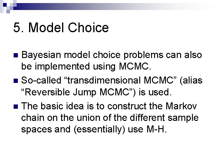
5. Model Choice Bayesian model choice problems can also be implemented using MCMC. n So-called “transdimensional MCMC” (alias “Reversible Jump MCMC”) is used. n The basic idea is to construct the Markov chain on the union of the different sample spaces and (essentially) use M-H. n

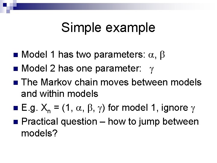
Simple example Model 1 has two parameters: , n Model 2 has one parameter: n The Markov chain moves between models and within models n E. g. Xn = (1, , , ) for model 1, ignore n Practical question – how to jump between models? n

Contents 1. MCMC: overview and basics n 2. Example: Vaccine efficacy n 3. Data augmentation n 4. Example: SIR epidemic model n 5. Model choice n 6. Example: Norovirus outbreak n 7. Other topics n

6. Example: Norovirus outbreak Outbreak of gastroenteritis in summer 2001 at school in Derbyshire, England. A single strain of Norovirus found to be the causative agent. Believed to be person-to-person spread

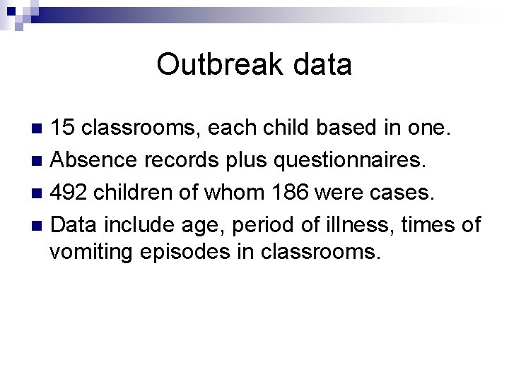
Outbreak data 15 classrooms, each child based in one. n Absence records plus questionnaires. n 492 children of whom 186 were cases. n Data include age, period of illness, times of vomiting episodes in classrooms. n

Question of interest n Does vomiting play a significant role in transmission? n Total of 15 vomiting episodes in classrooms.

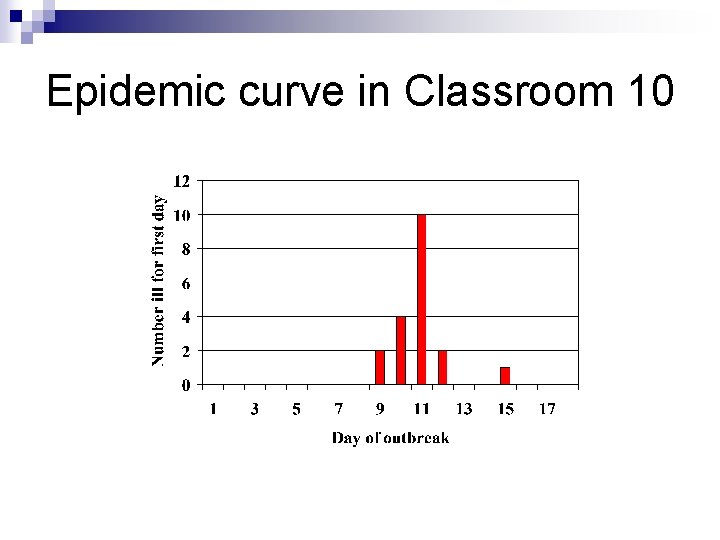
Epidemic curve in Classroom 10

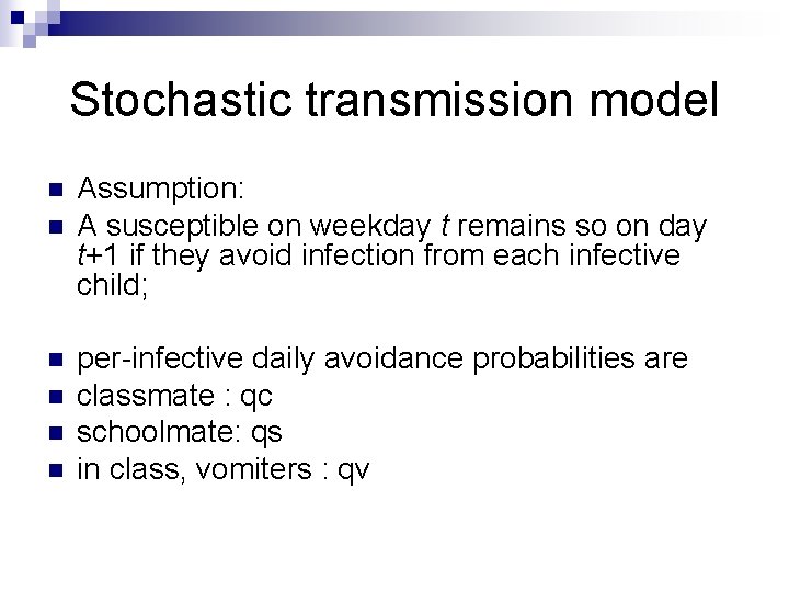
Stochastic transmission model n n n Assumption: A susceptible on weekday t remains so on day t+1 if they avoid infection from each infective child; per-infective daily avoidance probabilities are classmate : qc schoolmate: qs in class, vomiters : qv

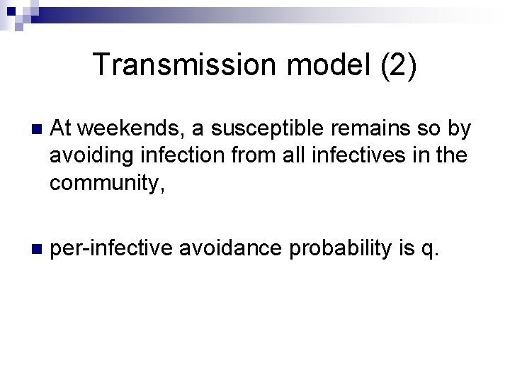
Transmission model (2) n At weekends, a susceptible remains so by avoiding infection from all infectives in the community, n per-infective avoidance probability is q.

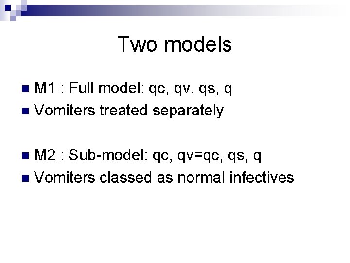
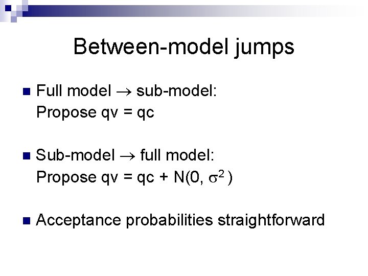
Two models M 1 : Full model: qc, qv, qs, q n Vomiters treated separately n M 2 : Sub-model: qc, qv=qc, qs, q n Vomiters classed as normal infectives n

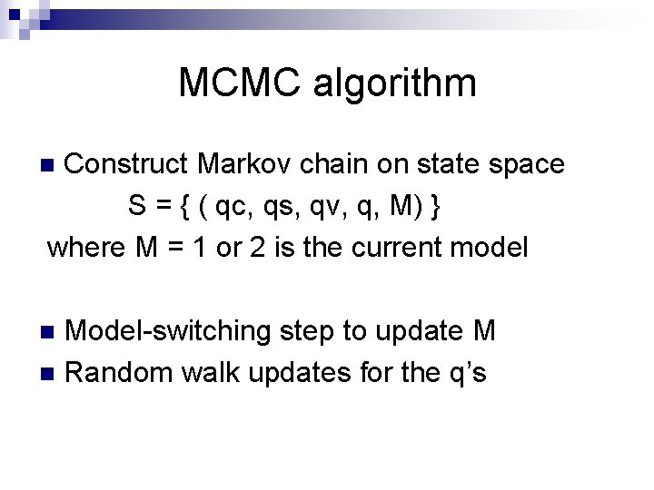
MCMC algorithm Construct Markov chain on state space S = { ( qc, qs, qv, q, M) } where M = 1 or 2 is the current model n Model-switching step to update M n Random walk updates for the q’s n

Between-model jumps n Full model sub-model: Propose qv = qc n Sub-model full model: Propose qv = qc + N(0, 2 ) n Acceptance probabilities straightforward

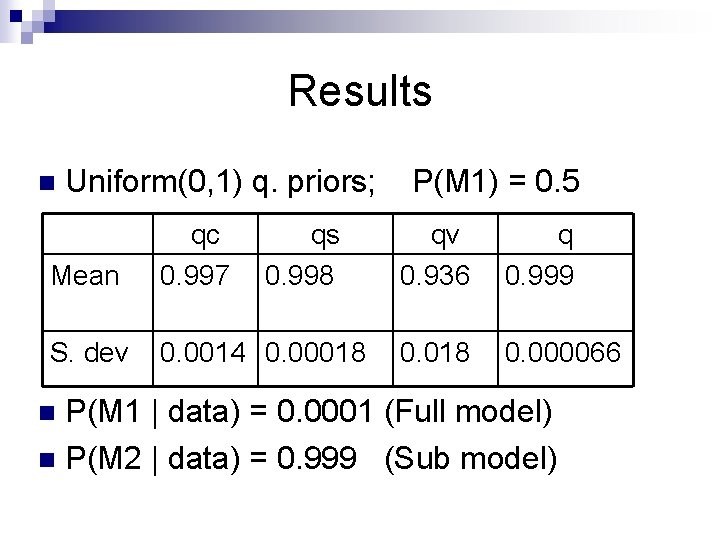
Results n Uniform(0, 1) q. priors; Mean qc 0. 997 qs 0. 998 S. dev 0. 0014 0. 00018 P(M 1) = 0. 5 qv 0. 936 q 0. 999 0. 018 0. 000066 P(M 1 | data) = 0. 0001 (Full model) n P(M 2 | data) = 0. 999 (Sub model) n

Contents 1. MCMC: overview and basics n 2. Example: Vaccine efficacy n 3. Data augmentation n 4. Example: SIR epidemic model n 5. Model choice n 6. Example: Norovirus outbreak n 7. Other topics n

7. Other topics 1. Improving algorithm performance n 2. Perfect simulation n 3. Some conclusions n

Improving algorithm performance Choose parameters to reduce correlation n Trade-off between ease of computation and mixing behaviour of chain n Choice of M-H proposal distributions n Choice of blocking schemes n

Perfect simulation Detecting convergence can be a real problem in practice. n Perfect simulation is a method for constructing a chain that is known to have converged by a certain time. n Unfortunately it is far less applicable than MCMC. n

Some conclusions MCMC methods are hugely powerful n The methods enable analysis of very complicated models n Sample-based methods easily permit exploration of both parameters and functions of parameters n Implementation is often relatively easy n Software available (e. g. BUGS) n