Maxwells microscopic equations gaussian units Classical theory Quantum

Maxwell’s microscopic equations (gaussian units): Classical theory: Quantum theory:

Maxwell’s macroscopic equations Macroscopic charge density and current averaged over a volume ΔV, where a 03 << ΔV << (2πc/ω)3 Gauss: Ampère: Gauss' law for magnetism: Faraday:

Currents and charge densities: External sources + internal sources We can distinguish three types of macroscopic internal sources: Conduction by free charges, polarization (‘bound charge) and magnetization Purely transversal

Gauss: Ampère: External field Magnetic field strength Gauss: Ampère:

Properties of the Medium, Linear Response to an externally applied electric field in homogeneous matter: External currents are zero inside sample, Homogeneous sample: Ampère’s law: Plane waves

Induced current: free charges+polarization+magnetization

Current response to an externally applied electric field in homogeneous matter:

Kramers Kronig Relations

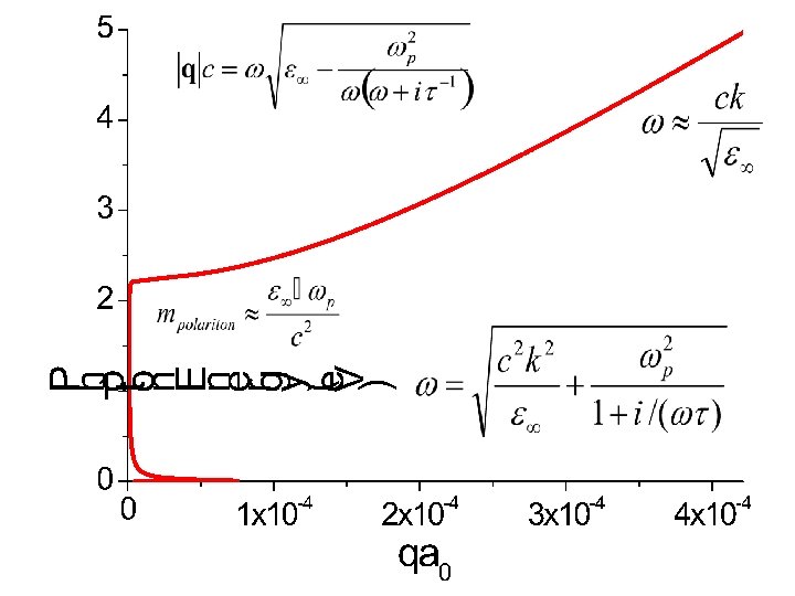
Transverse EM+matter waves: Polaritons Wave equation Polaritons: Transverse polarized waves of Matter & EM field Substituton of this solution in the wave equation provides the dispersion relation:

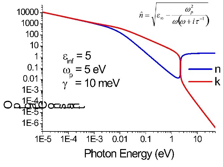
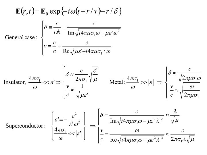
The polariton solitions in the solid have the form It is often convenient to use the optical constant in this expression, which has a real and imaginary part: Note, that n>0 and k>0. Also Im(ε)>0, but it is possible to have Re(ε)<0. If Im(ε)=0 and Re(ε)<0 it follows that k>0, but there is no dissipation!

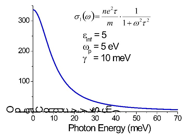
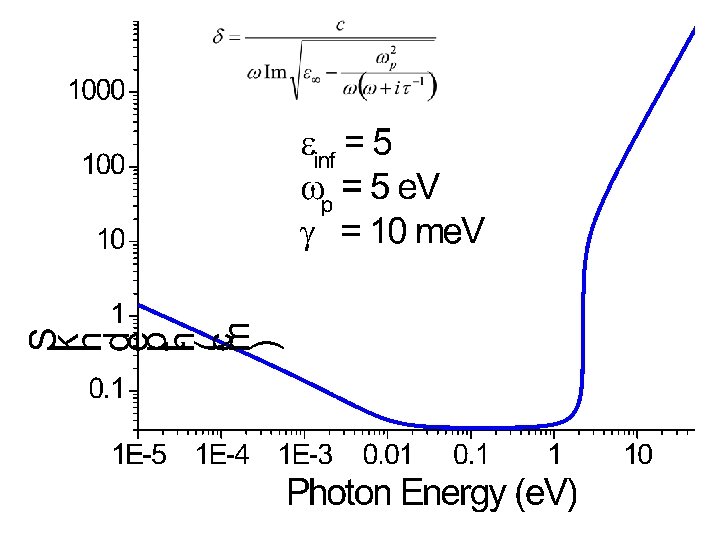
Case study: The Drude model

Optical techniques ellipsometry reflection Au evaporator Polarizer Sample sample transmission Analyzer Polarizer Sample Optical conductivity s 1(w) + i s 2(w)

Experimental ways to measure 1) In most cases only information can be obtained for q << 1/a 0 2) can be found by means of optical refraction, reflection, absorption, and polarization analysis.

Transverse EM+matter waves: Unless specified otherwise, we will from now on assume that

Reflection and transmission at a vacuum-sample interface Ei Et Er

Often the experiment provides the reflected intensity instead of the amplitude, and the phase of the reflected signal is in general difficult to measure. The reflection coefficient is: Kramers Kronig Relations are often used to get the phase of the reflectivity

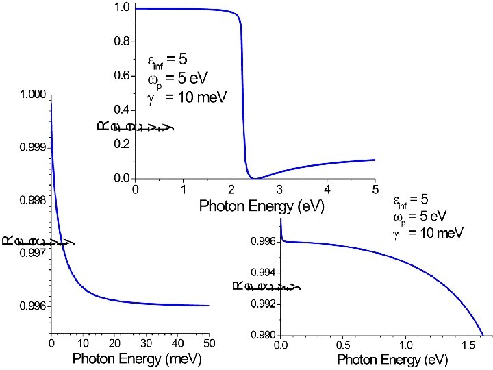
Example I : pure Bi

0 30 60 90 E (me. V)

Reflectivity at an oblique angle P-polarization: Ep is Parallel to the plane of reflection Ep Ep Hs a c b Hs

Reflectivity at an oblique angle Senkrecht (german) = Perpendicular S-polarization: Es is Senkrecht to the plane of reflection Hp Hp Es Es a c b

Nb. N Optically isotropic Normal incidence grazing incidence. Angle = 800 p-polarized light

Grazing incidence. Angle = 800 p-polarized light

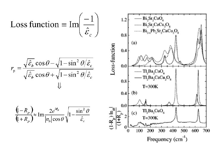
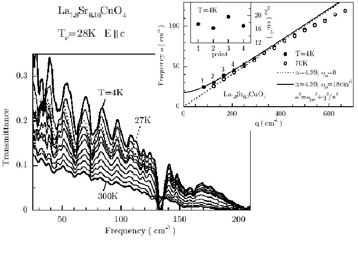
Josephson Coupled Planes d d Josephson Plasma Resonance at C L

Ree w Reflection normal to ac-plane Grazing incidence reflection of ab-plane 1 1 0 w

La 2 -x. Srx. Cu. O 4 Tl 2 Ba 2 Cu. O 6

Spectroscopic ellipsometry: Measurement of |rp/rs| and hp-hs e(w) = e 1(w) + 4 pi s 1(w)/w - self normalizing technique (no reference is required) - measures directly both real and imaginary parts of the dielectric function

Spectroscopic ellipsometry A 0 P a c b

Ellipsometry technique polariser analyser 2γ Ellipsometrie I) II) A 0

Ellipsometry technique polariser analyser 2γ Ellipsometrie I) II) A 0

Spectroscopic ellipsometry A 0 P a c b Aspnes theorem: Aspnes theorem

Bi 2212

ab-plane dielectric function corrected for c-axis admixture Pseudo ab-plane dielectric function

Experiment and ab-initio calculations

Thick wedged films:

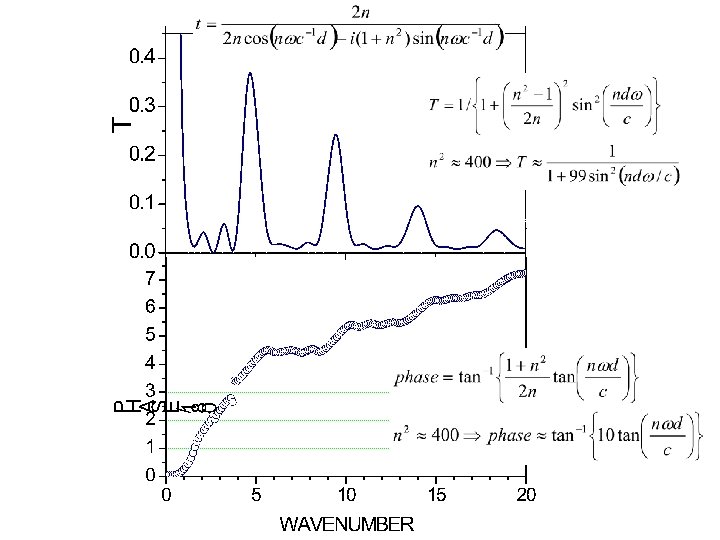
Weakly absorbing excitations in insulating YBa 2 Cu 3 O 6 No absorbtive features in R(w) Absorbtive features in T(w) M. U. Gruninger, 1999 Ph. D Thesis YBa 2 Cu 3 O 6

Optical Transmission

Thin films:

Thin films: 18 K 13 K 9 K 9 K 13 K Nb. N d=400 nm

Fused quartz Nd. Ga. O 3 KRS 5

Transmission Sr. Ti. O 3 Sr 0 10 20 30 40 50

THz time domain measurements Fabry-Perot etalon source detector

THz time domain measurements Fabry-Perot etalon source detector

THz transmission of Sr. Ti. O 3 intensity (a. u. ) Time domain 31 32 33 34 35 delay line (mm) 36 37

THz transmission of Sr. Ti. O 3 Time domain Frequency domain transmission intensity (a. u. ) 0. 1 31 32 33 34 35 36 37 10 -3 10 -5 0 10 20 30 40 wavenumber (cm-1) delay line (mm) Fourier transformation 50

Drude-Lorentz fit with Ref. FIT http: //optics. unige. ch/alexey/reffit. html

Transmission Direct measurement of the polariton w(q) relation 0 10 20 30 40 50