Maximum likelihood ML method Jarno Tuimala Thanks to

Maximum likelihood (ML) method Jarno Tuimala Thanks to James Mc. Inerney for the slides with a darker background!

Maximum likelihood • Historically a new method (Felsenstein, 1980’s) • ML assumes a model of sequence evolution • Using the model, ML method tries to answer the question: what is the likelihood (conditional probability) of observing these data given a certain model

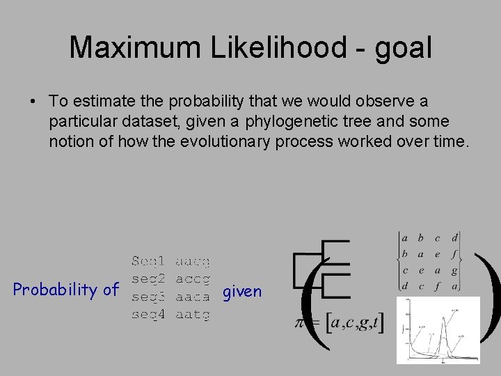
Maximum Likelihood - goal • To estimate the probability that we would observe a particular dataset, given a phylogenetic tree and some notion of how the evolutionary process worked over time. Probability of given ( )

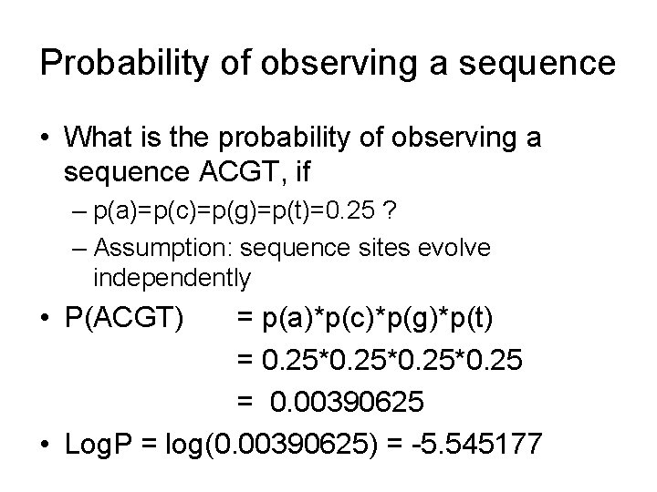
Probability of observing a sequence • What is the probability of observing a sequence ACGT, if – p(a)=p(c)=p(g)=p(t)=0. 25 ? – Assumption: sequence sites evolve independently • P(ACGT) = p(a)*p(c)*p(g)*p(t) = 0. 25*0. 25 = 0. 00390625 • Log. P = log(0. 00390625) = -5. 545177

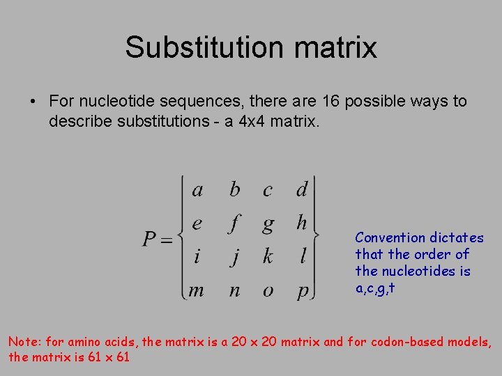
Substitution matrix • For nucleotide sequences, there are 16 possible ways to describe substitutions - a 4 x 4 matrix. Convention dictates that the order of the nucleotides is a, c, g, t Note: for amino acids, the matrix is a 20 x 20 matrix and for codon-based models, the matrix is 61 x 61

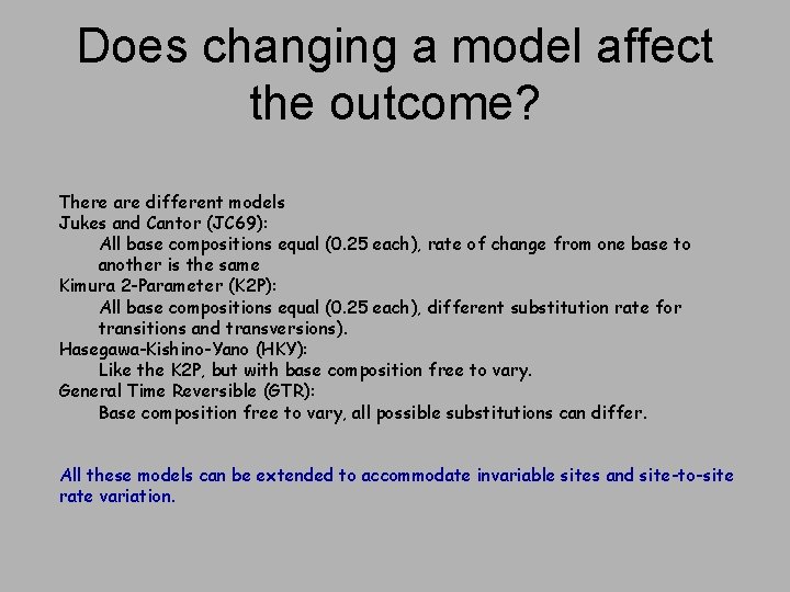
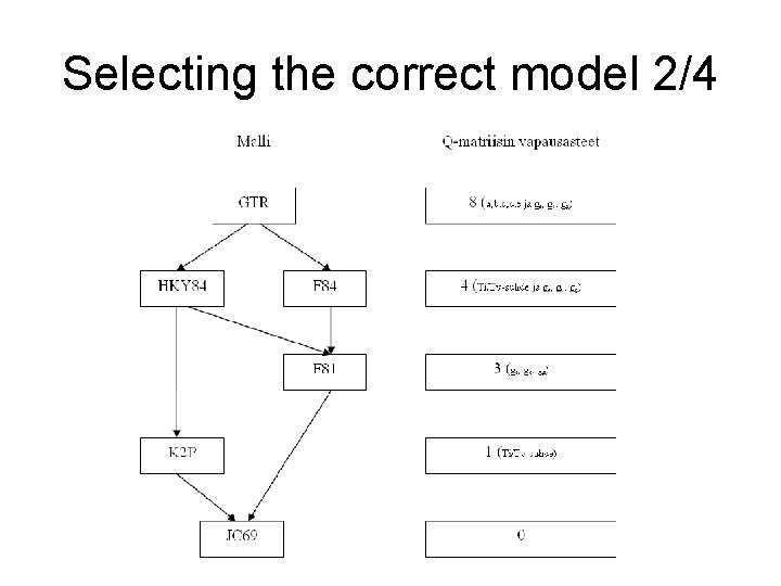
Does changing a model affect the outcome? There are different models Jukes and Cantor (JC 69): All base compositions equal (0. 25 each), rate of change from one base to another is the same Kimura 2 -Parameter (K 2 P): All base compositions equal (0. 25 each), different substitution rate for transitions and transversions). Hasegawa-Kishino-Yano (HKY): Like the K 2 P, but with base composition free to vary. General Time Reversible (GTR): Base composition free to vary, all possible substitutions can differ. All these models can be extended to accommodate invariable sites and site-to-site rate variation.

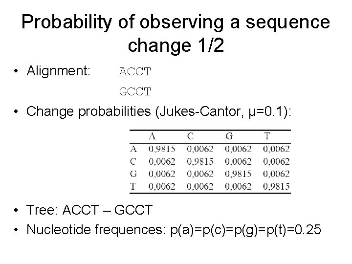
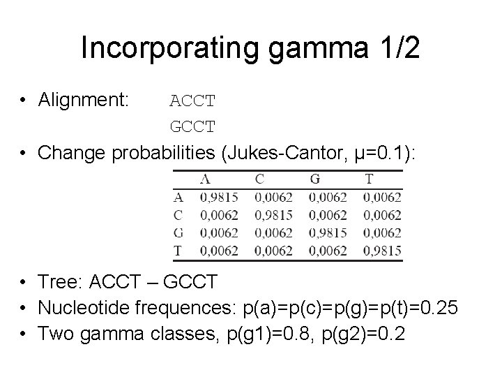
Probability of observing a sequence change 1/2 • Alignment: ACCT GCCT • Change probabilities (Jukes-Cantor, μ=0. 1): • Tree: ACCT – GCCT • Nucleotide frequences: p(a)=p(c)=p(g)=p(t)=0. 25

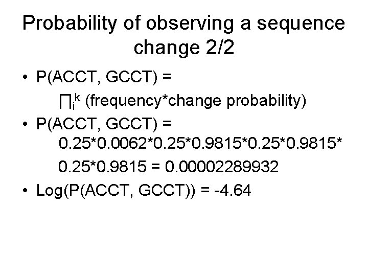
Probability of observing a sequence change 2/2 • P(ACCT, GCCT) = ∏ik (frequency*change probability) • P(ACCT, GCCT) = 0. 25*0. 0062*0. 25*0. 9815* 0. 25*0. 9815 = 0. 00002289932 • Log(P(ACCT, GCCT)) = -4. 64

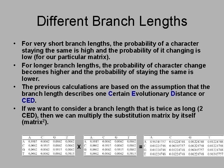
Different Branch Lengths • For very short branch lengths, the probability of a character staying the same is high and the probability of it changing is low (for our particular matrix). • For longer branch lengths, the probability of character change becomes higher and the probability of staying the same is lower. • The previous calculations are based on the assumption that the branch length describes one Certain Evolutionary Distance or CED. • If we want to consider a branch length that is twice as long (2 CED), then we can multiply the substitution matrix by itself (matrix 2). X =

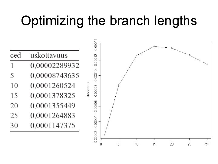
Optimizing the branch lengths

Invariable sites • For a given dataset we can assume that a certain proportion of sites are not free to vary - purifying selection (related to function) prevents these sites from changing). • We can therefore observe invariable positions either because they are under this selective constraint or because they have not had a chance to vary or because there is homoplasy in the dataset and a reversal (say) has caused the site to appear constant. • The likelihood that a site is invariable can be calculated by incorporating this possibility into our model and calculating for every site the likelihood that it is an invariable site. • It might improve the likelihood of the dataset if we remove a certain proportion of invariable sites (in a way that is analogous to the preceding discussion).

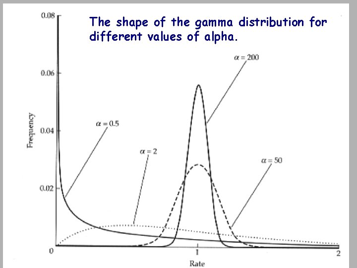
Variable sites • Obviously other sites in the dataset are free to vary. • Selection intensity on these sites is rarely uniform, so it is desirable to model site-by-site rate variation. • This is done in two ways: – site specific (codon position, or alpha helix etc. ) – using a discrete approximation to a continuous distribution (gamma distribution). • Again, these variables are modeled over all possibilities of sequence change over all possibilities of branch length over all possibilities of tree topology.

The shape of the gamma distribution for different values of alpha.

Incorporating gamma 1/2 • Alignment: ACCT GCCT • Change probabilities (Jukes-Cantor, μ=0. 1): • Tree: ACCT – GCCT • Nucleotide frequences: p(a)=p(c)=p(g)=p(t)=0. 25 • Two gamma classes, p(g 1)=0. 8, p(g 2)=0. 2

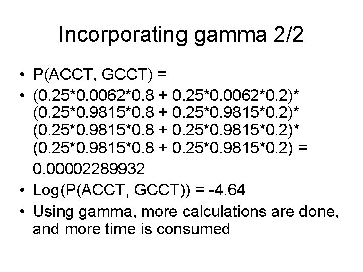
Incorporating gamma 2/2 • P(ACCT, GCCT) = • (0. 25*0. 0062*0. 8 + 0. 25*0. 0062*0. 2)* (0. 25*0. 9815*0. 8 + 0. 25*0. 9815*0. 2) = 0. 00002289932 • Log(P(ACCT, GCCT)) = -4. 64 • Using gamma, more calculations are done, and more time is consumed

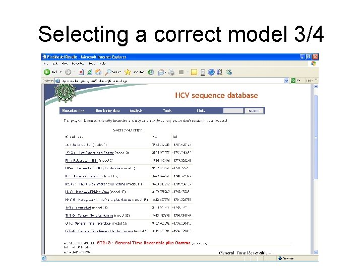
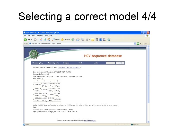
Selecting the correct model 1/4 • It was previously pointed out that parsimony can be inconsistent. • ML can be inconsistent too! • If the model used in the ML analysis is incorrect, the method might become inconsistent. • Before analysis, the correct model should be selected.

Selecting the correct model 2/4

Selecting a correct model 3/4

Selecting a correct model 4/4

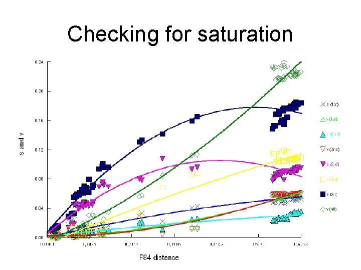
Checking for saturation

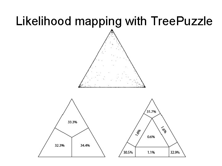
Likelihood mapping with Tree. Puzzle

Practical issues • There is an ML equivalent to Wagner method for generating initial trees, but it is very slow. • Many programs create an initial tree using parsimony or distance methods or use a completely random tree. • Search strategy is similar to parsimony: – 100 RAS + TBR for small dataset – In addition, simulated annealing can be used for larger datasets