Maximum Likelihood Method MLM Does this procedure make

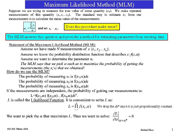
Maximum Likelihood Method (MLM) Does this procedure make sense? The MLM answers this question and provides a method for estimating parameters from existing data. We drop the dxn since it is just proportionality constant 880. P 20 Winter 2006 Richard Kass 1

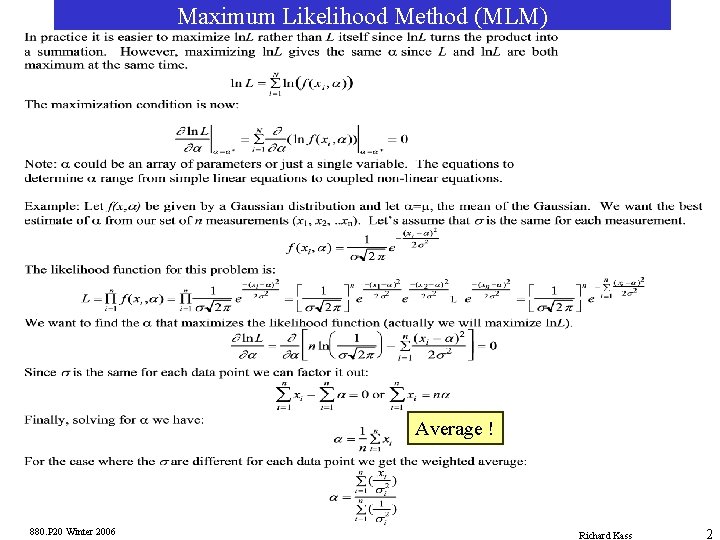
Maximum Likelihood Method (MLM) Average ! 880. P 20 Winter 2006 Richard Kass 2

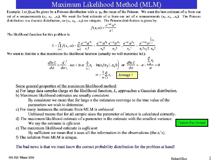
Maximum Likelihood Method (MLM) Average ! Cramer-Rao bound 880. P 20 Winter 2006 Richard Kass 3

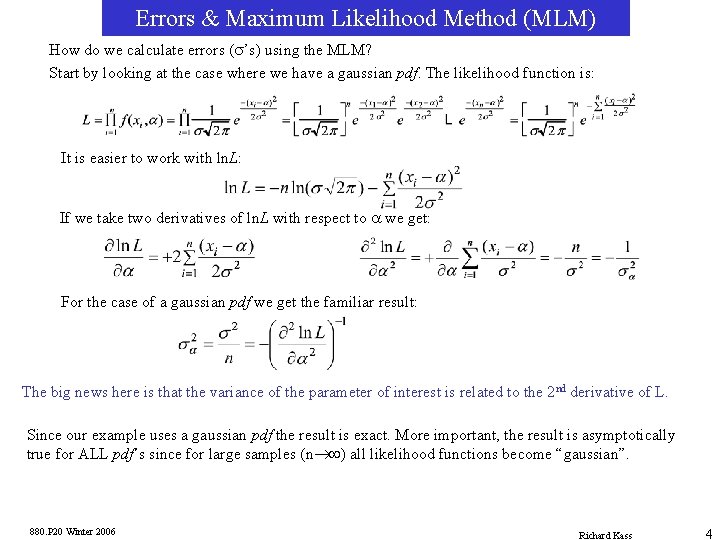
Errors & Maximum Likelihood Method (MLM) How do we calculate errors (s’s) using the MLM? Start by looking at the case where we have a gaussian pdf. The likelihood function is: It is easier to work with ln. L: If we take two derivatives of ln. L with respect to a we get: For the case of a gaussian pdf we get the familiar result: The big news here is that the variance of the parameter of interest is related to the 2 nd derivative of L. Since our example uses a gaussian pdf the result is exact. More important, the result is asymptotically true for ALL pdf’s since for large samples (n®¥) all likelihood functions become “gaussian”. 880. P 20 Winter 2006 Richard Kass 4

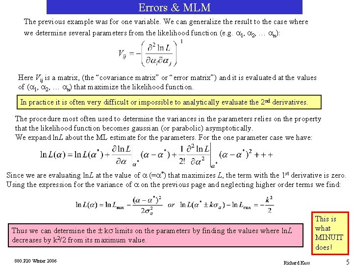
Errors & MLM The previous example was for one variable. We can generalize the result to the case where we determine several parameters from the likelihood function (e. g. a 1, a 2, … an): Here Vij is a matrix, (the “covariance matrix” or “error matrix”) and it is evaluated at the values of (a 1, a 2, … an) that maximize the likelihood function. In practice it is often very difficult or impossible to analytically evaluate the 2 nd derivatives. The procedure most often used to determine the variances in the parameters relies on the property that the likelihood function becomes gaussian (or parabolic) asymptotically. We expand ln. L about the ML estimate for the parameters. For the one parameter case we have: Since we are evaluating ln. L at the value of a (=a*) that maximizes L, the term with the 1 st derivative is zero. Using the expression for the variance of a on the previous page and neglecting higher order terms we find: Thus we can determine the ± ks limits on the parameters by finding the values where ln. L decreases by k 2/2 from its maximum value. 880. P 20 Winter 2006 Richard Kass This is what MINUIT does! 5

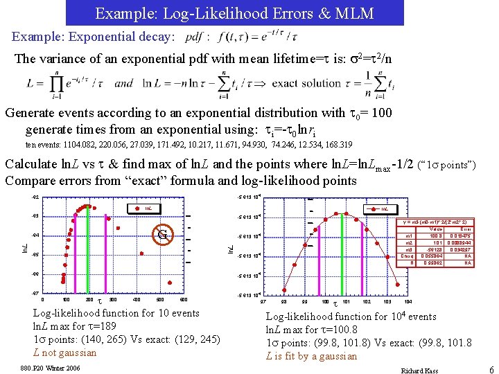
Example: Log-Likelihood Errors & MLM Example: Exponential decay: The variance of an exponential pdf with mean lifetime=t is: s 2=t 2/n Generate events according to an exponential distribution with t 0= 100 generate times from an exponential using: ti=-t 0 lnri ten events: 1104. 082, 220. 056, 27. 039, 171. 492, 10. 217, 11. 671, 94. 930, 74. 246, 12. 534, 168. 319 Calculate ln. L vs t & find max of ln. L and the points where ln. L=ln. Lmax-1/2 (“ 1 s points”) Compare errors from “exact” formula and log-likelihood points -5. 613 10 4 -62 ln. L -5. 613 10 4 -63 G x -5. 613 10 4 ln. L -64 y = m 3 -(m 0 -m 1)^ 2/(2*m 2^ 2) Value Error m 1 100. 8 0. 013475 m 2 1. 01 0. 0088944 m 3 -56128 0. 034297 Chisq 0. 055864 NA R 0. 99862 NA -65 -66 -5. 613 10 4 -67 0 100 200 t 300 400 500 600 Log-likelihood function for 10 events ln. L max for t=189 1 s points: (140, 265) Vs exact: (129, 245) L not gaussian 880. P 20 Winter 2006 -5. 613 10 4 97 98 99 100 t 101 102 103 104 Log-likelihood function for 104 events ln. L max for t=100. 8 1 s points: (99. 8, 101. 8) Vs exact: (99. 8, 101. 8 L is fit by a gaussian Richard Kass 6

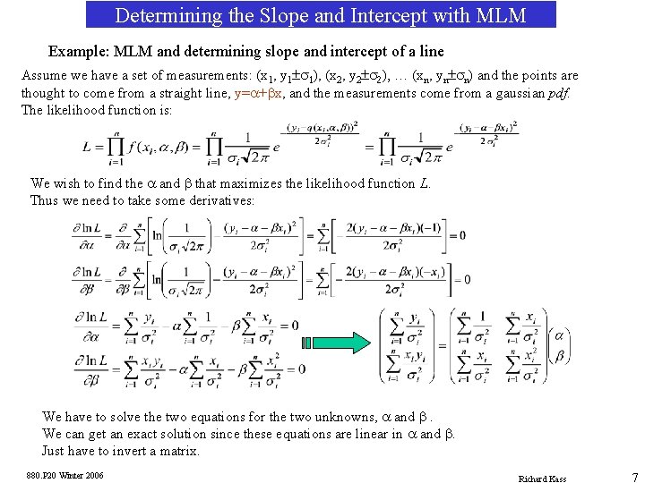
Determining the Slope and Intercept with MLM Example: MLM and determining slope and intercept of a line Assume we have a set of measurements: (x 1, y 1±s 1), (x 2, y 2±s 2), … (xn, yn±sn) and the points are thought to come from a straight line, y=a+bx, and the measurements come from a gaussian pdf. The likelihood function is: We wish to find the a and b that maximizes the likelihood function L. Thus we need to take some derivatives: We have to solve the two equations for the two unknowns, a and b. We can get an exact solution since these equations are linear in a and b. Just have to invert a matrix. 880. P 20 Winter 2006 Richard Kass 7

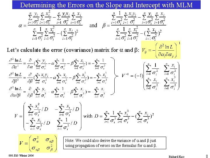
Determining the Errors on the Slope and Intercept with MLM Let’s calculate the error (covariance) matrix for a and b: Note: We could also derive the variance of a and b just using propagation of errors on the formulas for a and b. 880. P 20 Winter 2006 Richard Kass 8

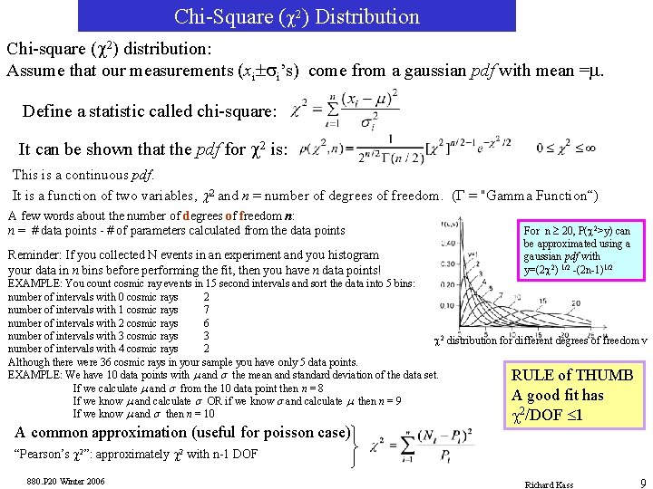
Chi-Square (c 2) Distribution Chi-square (c 2) distribution: Assume that our measurements (xi±si’s) come from a gaussian pdf with mean =m. Define a statistic called chi-square: It can be shown that the pdf for c 2 is: This is a continuous pdf. It is a function of two variables, c 2 and n = number of degrees of freedom. (G = "Gamma Function“) A few words about the number of degrees of freedom n: n = # data points - # of parameters calculated from the data points Reminder: If you collected N events in an experiment and you histogram your data in n bins before performing the fit, then you have n data points! For n ³ 20, P(c 2>y) can be approximated using a gaussian pdf with y=(2 c 2) 1/2 -(2 n-1)1/2 EXAMPLE: You count cosmic ray events in 15 second intervals and sort the data into 5 bins: number of intervals with 0 cosmic rays 2 number of intervals with 1 cosmic rays 7 number of intervals with 2 cosmic rays 6 number of intervals with 3 cosmic rays 3 c 2 distribution for different degrees of freedom v number of intervals with 4 cosmic rays 2 Although there were 36 cosmic rays in your sample you have only 5 data points. EXAMPLE: We have 10 data points with m and s the mean and standard deviation of the data set. RULE of THUMB If we calculate m and s from the 10 data point then n = 8 A good fit has If we know m and calculate s OR if we know s and calculate m then n = 9 If we know m and s then n = 10 c 2/DOF £ 1 A common approximation (useful for poisson case) “Pearson’s c 2”: approximately c 2 with n-1 DOF 880. P 20 Winter 2006 Richard Kass 9

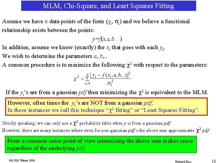
MLM, Chi-Square, and Least Squares Fitting Assume we have n data points of the form (yi, si) and we believe a functional relationship exists between the points: y=f(x, a, b…) In addition, assume we know (exactly) the xi that goes with each yi. We wish to determine the parameters a, b, . . A common procedure is to minimize the following c 2 with respect to the parameters: If the yi’s are from a gaussian pdf then minimizing the c 2 is equivalent to the MLM. However, often times the yi’s are NOT from a gaussian pdf. In these instances we call this technique “c 2 fitting” or “Least Squares Fitting”. Strictly speaking, we can only use a c 2 probability table when y is from a gaussian pdf. However, there are many instances where even for non-gaussian pdf’s the above sum approximates c 2 pdf. From a common sense point of view minimizing the above sum makes sense regardless of the underlying pdf. 880. P 20 Winter 2006 Richard Kass 10

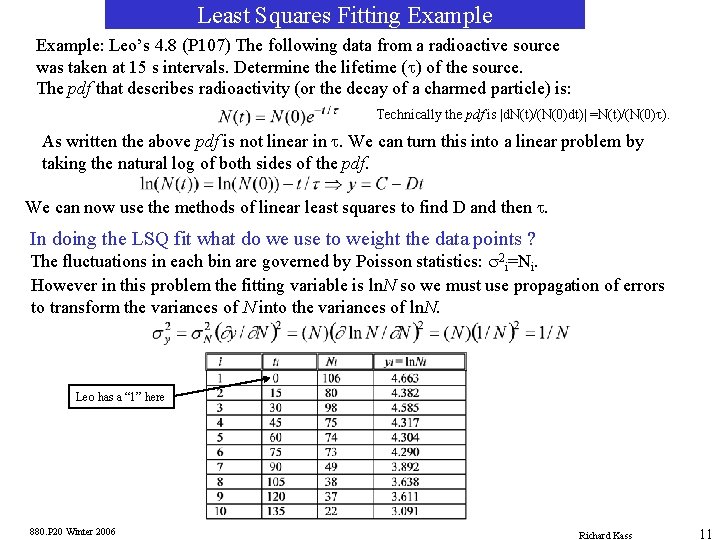
Least Squares Fitting Example: Leo’s 4. 8 (P 107) The following data from a radioactive source was taken at 15 s intervals. Determine the lifetime (t) of the source. The pdf that describes radioactivity (or the decay of a charmed particle) is: Technically the pdf is |d. N(t)/(N(0)dt)| =N(t)/(N(0)t). As written the above pdf is not linear in t. We can turn this into a linear problem by taking the natural log of both sides of the pdf. We can now use the methods of linear least squares to find D and then t. In doing the LSQ fit what do we use to weight the data points ? The fluctuations in each bin are governed by Poisson statistics: s 2 i=Ni. However in this problem the fitting variable is ln. N so we must use propagation of errors to transform the variances of N into the variances of ln. N. Leo has a “ 1” here 880. P 20 Winter 2006 Richard Kass 11

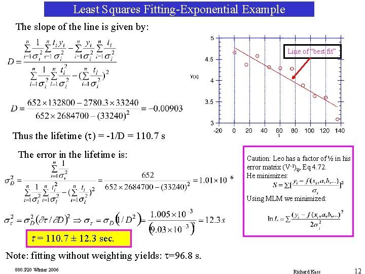
Least Squares Fitting-Exponential Example The slope of the line is given by: Line of “best fit” Thus the lifetime (t) = -1/D = 110. 7 s The error in the lifetime is: Caution: Leo has a factor of ½ in his error matrix (V-1)ij, Eq 4. 72. He minimizes: Using MLM we minimized: t = 110. 7 ± 12. 3 sec. Note: fitting without weighting yields: t=96. 8 s. 880. P 20 Winter 2006 Richard Kass 12

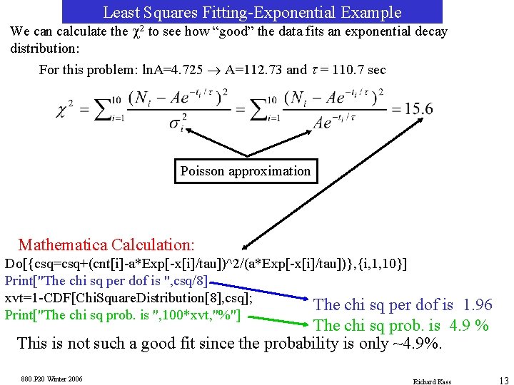
Least Squares Fitting-Exponential Example We can calculate the c 2 to see how “good” the data fits an exponential decay distribution: For this problem: ln. A=4. 725 ® A=112. 73 and t = 110. 7 sec Poisson approximation Mathematica Calculation: Do[{csq=csq+(cnt[i]-a*Exp[-x[i]/tau])^2/(a*Exp[-x[i]/tau])}, {i, 1, 10}] Print["The chi sq per dof is ", csq/8] xvt=1 -CDF[Chi. Square. Distribution[8], csq]; The chi sq per dof is 1. 96 Print["The chi sq prob. is ", 100*xvt, "%"] The chi sq prob. is 4. 9 % This is not such a good fit since the probability is only ~4. 9%. 880. P 20 Winter 2006 Richard Kass 13

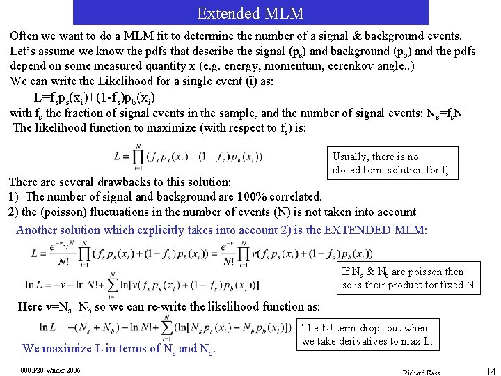
Extended MLM Often we want to do a MLM fit to determine the number of a signal & background events. Let’s assume we know the pdfs that describe the signal (ps) and background (pb) and the pdfs depend on some measured quantity x (e. g. energy, momentum, cerenkov angle. . ) We can write the Likelihood for a single event (i) as: L=fsps(xi)+(1 -fs)pb(xi) with fs the fraction of signal events in the sample, and the number of signal events: Ns=fs. N The likelihood function to maximize (with respect to fs) is: Usually, there is no closed form solution for fs There are several drawbacks to this solution: 1) The number of signal and background are 100% correlated. 2) the (poisson) fluctuations in the number of events (N) is not taken into account Another solution which explicitly takes into account 2) is the EXTENDED MLM: If Ns & Nb are poisson then so is their product for fixed N Here v=Ns+Nb so we can re-write the likelihood function as: We maximize L in terms of Ns and Nb. 880. P 20 Winter 2006 The N! term drops out when we take derivatives to max L. Richard Kass 14

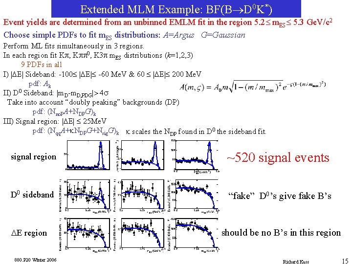
Extended MLM Example: BF(B®D 0 K*) Event yields are determined from an unbinned EMLM fit in the region 5. 2£ m. ES£ 5. 3 Ge. V/c 2 Choose simple PDFs to fit m. ES distributions: A=Argus G=Gaussian Perform ML fits simultaneously in 3 regions. In each region fit Kp, Kpp 0, K 3 p m. ES distributions (k=1, 2, 3) 9 PDFs in all I) |DE| Sideband: -100£ |DE|£ -60 Me. V & 60 £ |DE|£ 200 Me. V pdf: Ak II) D 0 Sideband: |m. D-m. D, PDG|> 4 s Take into account “doubly peaking” backgrounds (DP) pdf: (Nno. PA+NDPG)k III) Signal region: |DE| £ 25 Me. V pdf: (Nqq. A+k. NDPG+Nsig. G)k k scales the NDP found in D 0 the sideband fit. signal region ~520 signal events D 0 sideband “fake” D 0’s give fake B’s DE region 880. P 20 Winter 2006 should be no B’s in this region Richard Kass 15