Maximum Likelihood Benjamin Neale Boulder Workshop 2012 We

Maximum Likelihood Benjamin Neale Boulder Workshop 2012

We will cover • Easy introduction to probability • Rules of probability • How to calculate likelihood for discrete outcomes • Confidence intervals in likelihood • Likelihood for continuous data

Starting simple • Let’s think about probability
Starting simple • Let’s think about probability – Coin tosses – Winning the lottery – Roll of the die – Roulette wheel
Starting simple • Let’s think about probability – Coin tosses – Winning the lottery – Roll of the die – Roulette wheel • Chance of an event occurring
Starting simple • Let’s think about probability – Coin tosses – Winning the lottery – Roll of the die – Roulette wheel • Chance of an event occurring • Written as P(event) = probability of the event
Simple probability calculations • To get comfortable with probability, let’s solve these problems: 1. Probability of rolling an even number on a six-sided die 2. Probability of pulling a club from a deck of cards
Simple probability calculations • To get comfortable with probability, let’s solve these problems: 1. Probability of rolling an even number on a six-sided die ½ or 0. 5 2. Probability of pulling a club from a deck of cards ¼ or 0. 25
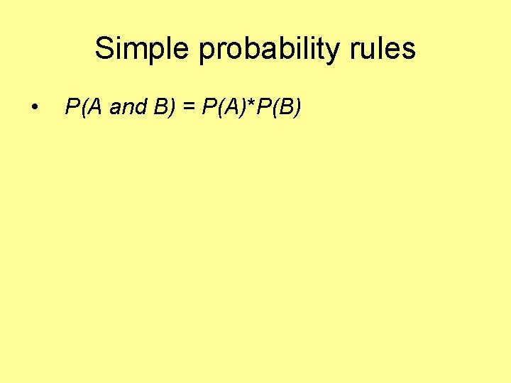
Simple probability rules • P(A and B) = P(A)*P(B)
Simple probability rules • P(A and B) = P(A)*P(B) – E. g. what is the probability of tossing 2 heads in a row?
Simple probability rules • P(A and B) = P(A)*P(B) – E. g. what is the probability of tossing 2 heads in a row? – A = Heads and B = Heads so,
Simple probability rules • P(A and B) = P(A)*P(B) – E. g. what is the probability of tossing 2 heads in a row? – A = Heads and B = Heads so, – P(A) = ½, P(B) = ½, P(A and B) = ¼
Simple probability rules • P(A and B) = P(A)*P(B) – E. g. what is the probability of tossing 2 heads in a row? – A = Heads and B = Heads so, – P(A) = ½, P(B) = ½, P(A and B) = ¼ *We assume independence
Simple probability rules cnt’d • P(A or B) = P(A) + P(B) – P(A and B)
Simple probability rules cnt’d • P(A or B) = P(A) + P(B) – P(A and B) – What is the probability of rolling a 1 or a 4?
Simple probability rules cnt’d • P(A or B) = P(A) + P(B) – P(A and B) – What is the probability of rolling a 1 or a 4? – A = rolling a 1 and B = rolling a 4
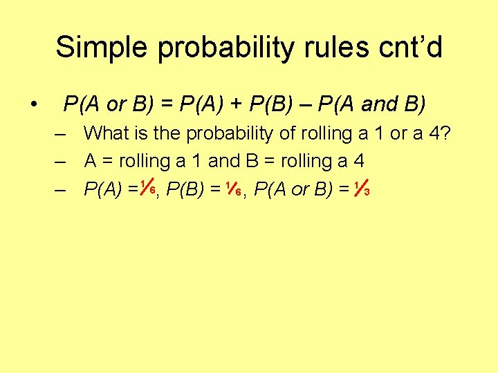
Simple probability rules cnt’d • P(A or B) = P(A) + P(B) – P(A and B) – What is the probability of rolling a 1 or a 4? – A = rolling a 1 and B = rolling a 4 1 1 6 – P(A) = , P(B) = , P(A or B) = 1 3 6
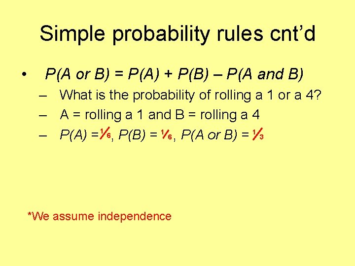
Simple probability rules cnt’d • P(A or B) = P(A) + P(B) – P(A and B) – What is the probability of rolling a 1 or a 4? – A = rolling a 1 and B = rolling a 4 1 1 6 – P(A) = , P(B) = , P(A or B) = 1 3 6 *We assume independence
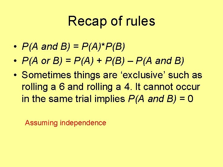
Recap of rules • P(A and B) = P(A)*P(B) • P(A or B) = P(A) + P(B) – P(A and B) • Sometimes things are ‘exclusive’ such as rolling a 6 and rolling a 4. It cannot occur in the same trial implies P(A and B) = 0 Assuming independence
Conditional probabilities • P(X | Y) = the probability of X occurring given Y.
Conditional probabilities • P(X | Y) = the probability of X occurring given Y. • Y can be another event (perhaps that predicts X)
Conditional probabilities • P(X | Y) = the probability of X occurring given Y. • Y can be another event (perhaps that predicts X) • Y can be a probability or set of probabilities
Conditional probabilities • Roll two dice in succession
Conditional probabilities • Roll two dice in succession • P(total = 10) = 1 12
Conditional probabilities • Roll two dice in succession • P(total = 10) = 1 12 • What is P(total = 10 | 1 st die = 5)?
Conditional probabilities • Roll two dice in succession • P(total = 10) = 1 12 • What is P(total = 10 | 1 st die = 5)? – P(total = 10 | 1 st die = 5) = 1 6
Binomial probabilities • Used for two conditions such as coin toss • Determine the chance of any outcome:
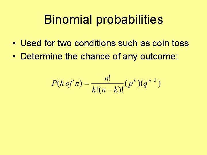
Binomial probabilities • Used for two conditions such as coin toss • Determine the chance of any outcome:
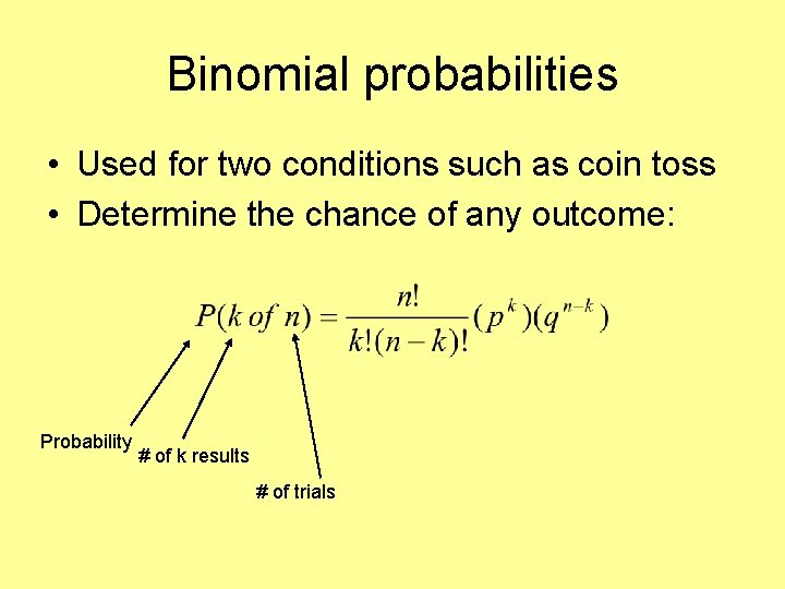
Binomial probabilities • Used for two conditions such as coin toss • Determine the chance of any outcome: Probability # of k results # of trials
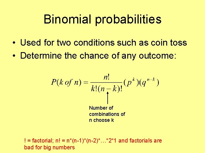
Binomial probabilities • Used for two conditions such as coin toss • Determine the chance of any outcome: Number of combinations of n choose k ! = factorial; n! = n*(n-1)*(n-2)*…*2*1 and factorials are bad for big numbers
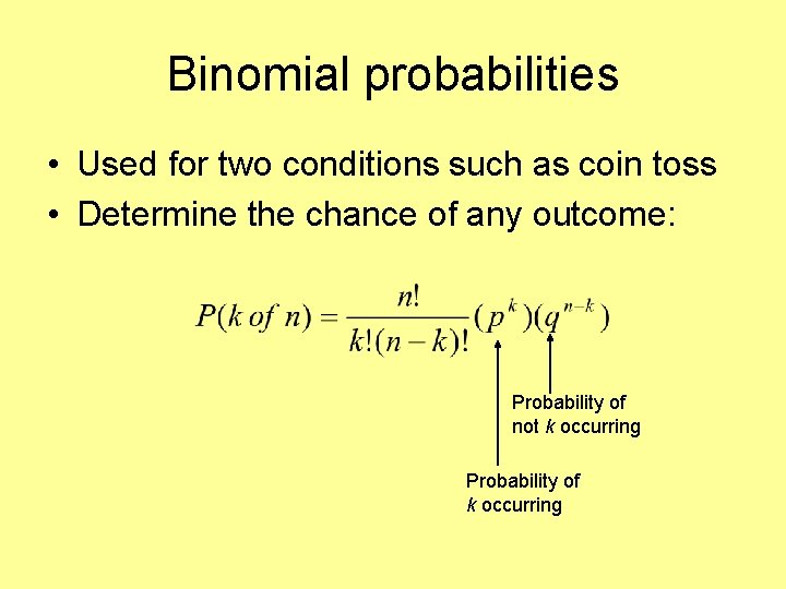
Binomial probabilities • Used for two conditions such as coin toss • Determine the chance of any outcome: Probability of not k occurring Probability of k occurring
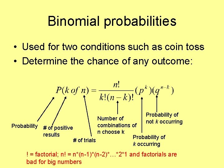
Binomial probabilities • Used for two conditions such as coin toss • Determine the chance of any outcome: Probability of Number of not k occurring combinations of # of positive n choose k results Probability of # of trials k occurring ! = factorial; n! = n*(n-1)*(n-2)*…*2*1 and factorials are bad for big numbers
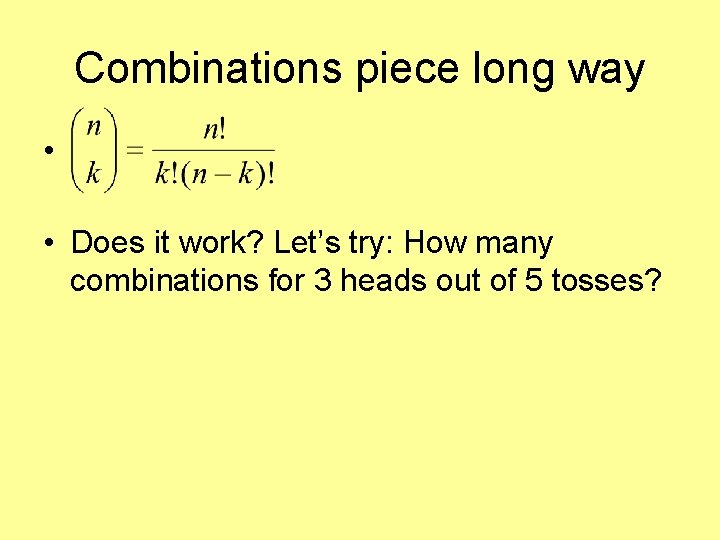
Combinations piece long way • • Does it work? Let’s try: How many combinations for 3 heads out of 5 tosses?
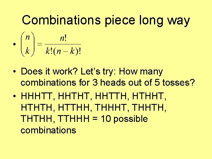
Combinations piece long way • • Does it work? Let’s try: How many combinations for 3 heads out of 5 tosses? • HHHTT, HHTHT, HHTTH, HTHHT, HTHTH, HTTHH, THHHT, THHTH, THTHH, TTHHH = 10 possible combinations
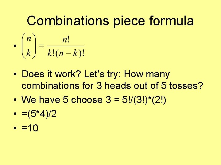
Combinations piece formula • • Does it work? Let’s try: How many combinations for 3 heads out of 5 tosses? • We have 5 choose 3 = 5!/(3!)*(2!) • =(5*4)/2 • =10
Probability roundup • We assumed the ‘true’ parameter values – E. g. P(Heads) = P(Tails) = ½
Probability roundup • We assumed the ‘true’ parameter values – E. g. P(Heads) = P(Tails) = ½ • What happens if we have data and want to determine the parameter values?
Probability roundup • We assumed the ‘true’ parameter values – E. g. P(Heads) = P(Tails) = ½ • • What happens if we have data and want to determine the parameter values? Likelihood works the other way round: what is the probability of the observed data given parameter values?
Concrete example • Likelihood aims to calculate the range of probabilities for observed data, assuming different parameter values.
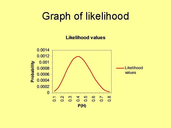
Concrete example • Likelihood aims to calculate the range of probabilities for observed data, assuming different parameter values. • The set of probabilities is referred to as a likelihood surface
Concrete example • Likelihood aims to calculate the range of probabilities for observed data, assuming different parameter values. • The set of probabilities is referred to as a likelihood surface • We’re going to generate the likelihood surface for a coin tossing experiment
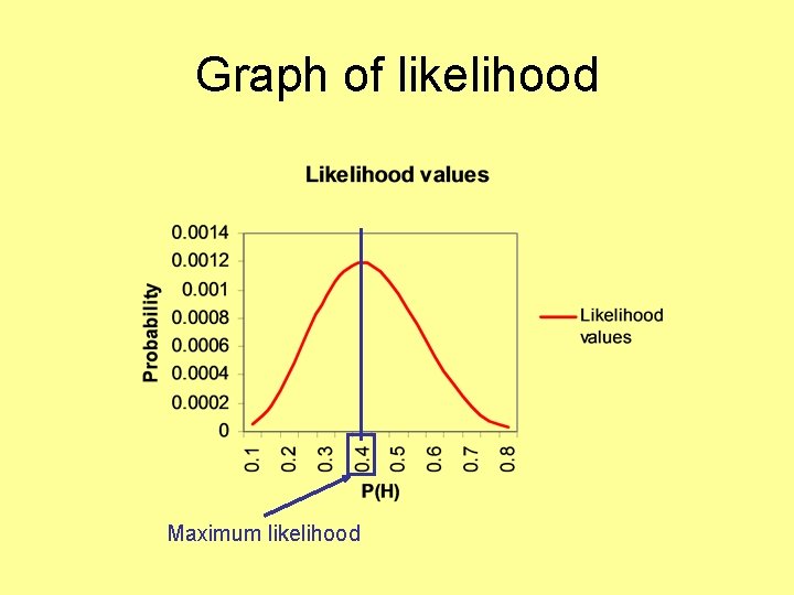
Concrete example • Likelihood aims to calculate the range of probabilities for observed data, assuming different parameter values. • The set of probabilities is referred to as a likelihood surface • We’re going to generate the likelihood surface for a coin tossing experiment • The set of parameter values with the best probability is the maximum likelihood

Coin tossing • I tossed a coin 10 times and get 4 heads and 6 tails

Coin tossing • I tossed a coin 10 times and get 4 heads and 6 tails • From this data, what does likelihood estimate the chance of heads and tails for this coin?
Coin tossing • I tossed a coin 10 times and get 4 heads and 6 tails • From this data, what does likelihood estimate the chance of heads and tails for this coin? • We’re going to calculate: – P(4 heads out of 10 tosses| P(H) = *) – where star takes on a range of values
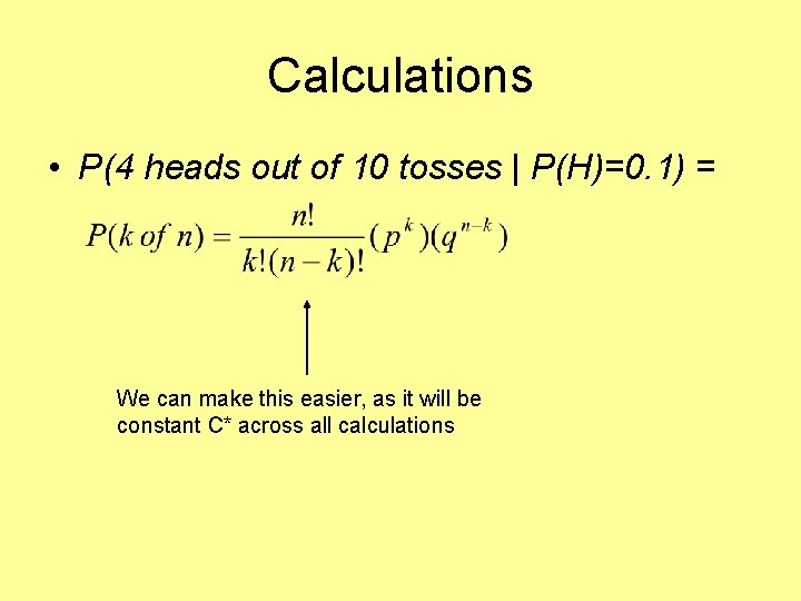
Calculations • P(4 heads out of 10 tosses | P(H)=0. 1) = We can make this easier, as it will be constant C* across all calculations
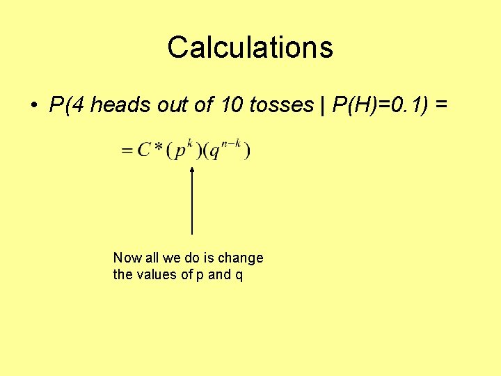
Calculations • P(4 heads out of 10 tosses | P(H)=0. 1) = Now all we do is change the values of p and q
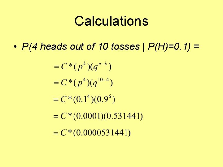
Calculations • P(4 heads out of 10 tosses | P(H)=0. 1) =
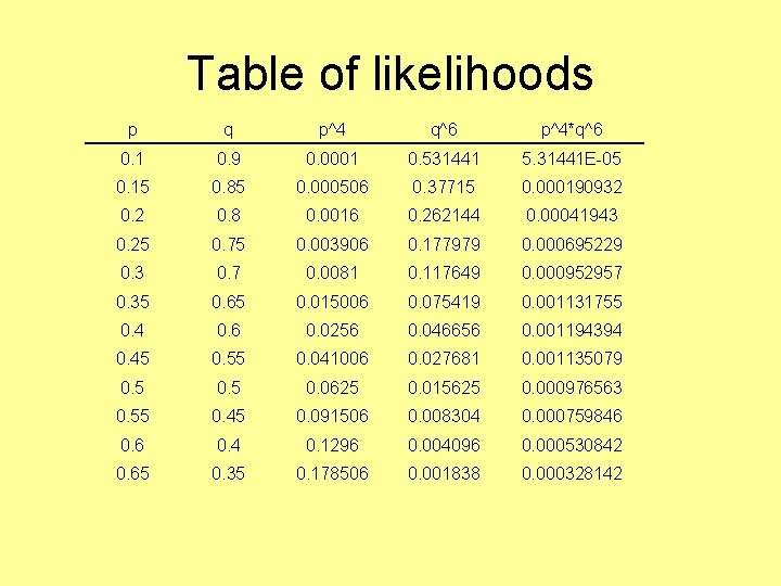
Table of likelihoods p q p^4 q^6 p^4*q^6 0. 1 0. 9 0. 0001 0. 531441 5. 31441 E-05 0. 15 0. 85 0. 000506 0. 37715 0. 000190932 0. 8 0. 0016 0. 262144 0. 00041943 0. 25 0. 75 0. 003906 0. 177979 0. 000695229 0. 3 0. 7 0. 0081 0. 117649 0. 000952957 0. 35 0. 65 0. 015006 0. 075419 0. 001131755 0. 4 0. 6 0. 0256 0. 046656 0. 001194394 0. 45 0. 55 0. 041006 0. 027681 0. 001135079 0. 5 0. 0625 0. 015625 0. 000976563 0. 55 0. 45 0. 091506 0. 008304 0. 000759846 0. 4 0. 1296 0. 004096 0. 000530842 0. 65 0. 35 0. 178506 0. 001838 0. 000328142
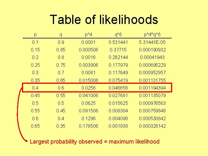
Table of likelihoods p q p^4 q^6 p^4*q^6 0. 1 0. 9 0. 0001 0. 531441 5. 31441 E-05 0. 15 0. 85 0. 000506 0. 37715 0. 000190932 0. 8 0. 0016 0. 262144 0. 00041943 0. 25 0. 75 0. 003906 0. 177979 0. 000695229 0. 3 0. 7 0. 0081 0. 117649 0. 000952957 0. 35 0. 65 0. 015006 0. 075419 0. 001131755 0. 4 0. 6 0. 0256 0. 046656 0. 001194394 0. 45 0. 55 0. 041006 0. 027681 0. 001135079 0. 5 0. 0625 0. 015625 0. 000976563 0. 55 0. 45 0. 091506 0. 008304 0. 000759846 0. 4 0. 1296 0. 004096 0. 000530842 0. 65 0. 35 0. 178506 0. 001838 0. 000328142 Largest probability observed = maximum likelihood
Graph of likelihood
Graph of likelihood Maximum likelihood
Formal likelihood for discrete outcomes • The binomial example can be expanded for any number of discrete outcomes:
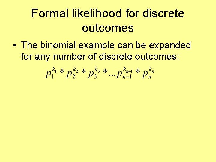
Formal likelihood for discrete outcomes • The binomial example can be expanded for any number of discrete outcomes:
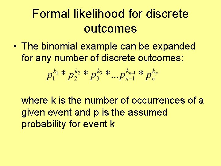
Formal likelihood for discrete outcomes • The binomial example can be expanded for any number of discrete outcomes: where k is the number of occurrences of a given event and p is the assumed probability for event k
Testing in maximum likelihood • We know how to choose the best model • How do we test for the best model? • When Fisher devised this approach, he noted that minus twice the difference in log likelihoods is distributed like a chi square with degrees of freedom equal to the number of parameters dropped or fixed
How does this test work? • Let’s test in our example, whether the chance of heads is significantly different from 0. 5 • We’ll use the likelihood ratio test • We are fixing 1 parameter, the estimate of heads • Note that P(tails) is constrained to be 1 -P(heads)
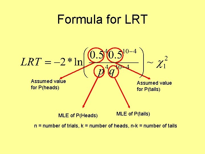
Formula for LRT Assumed value for P(heads) MLE of P(Heads) Assumed value for P(tails) MLE of P(tails) n = number of trials, k = number of heads, n-k = number of tails
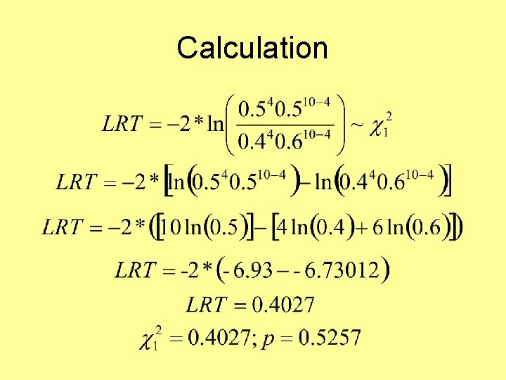
Calculation
LRT roundup • The key to the interpretation to the LRT is to understand what we are test • Formally, we are testing to determine whether the fit of the model is significantly worse • In layman’s terms: we are testing for the necessity of the parameter. A big chi square means the parameter is important
Confidence intervals • Now that we know how to estimate the parameter value and test significance we can determine MLE confidence intervals
Confidence intervals • Now that we know how to estimate the parameter value and test significance we can determine MLE confidence intervals • Anyone have any idea how we would generate CIs using MLE?
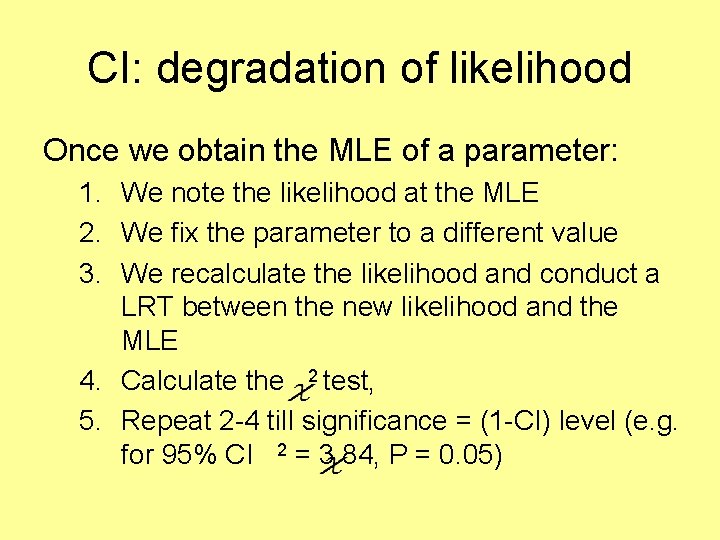
CI: degradation of likelihood Once we obtain the MLE of a parameter: 1. We note the likelihood at the MLE 2. We fix the parameter to a different value 3. We recalculate the likelihood and conduct a LRT between the new likelihood and the MLE 4. Calculate the 2 test, 5. Repeat 2 -4 till significance = (1 -CI) level (e. g. for 95% CI 2 = 3. 84, P = 0. 05)

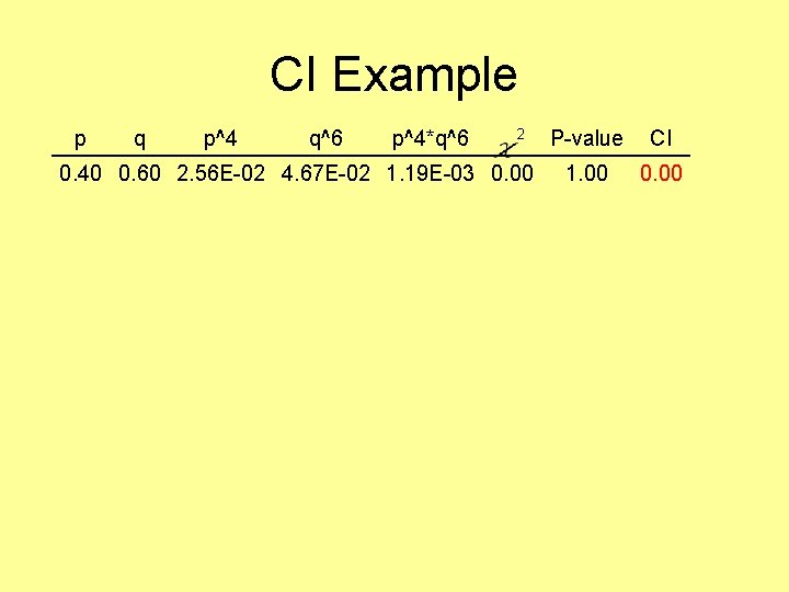
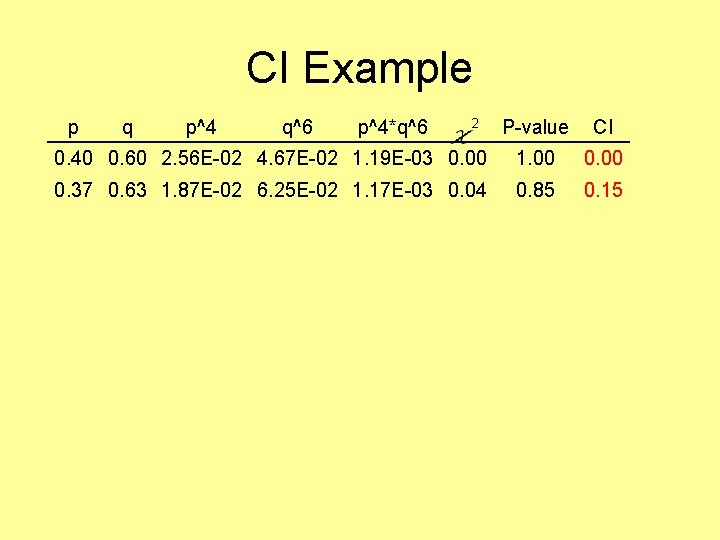
CI Example Returning to our trusty coin toss example 1. 2. 3. 4. Our MLE was P(Heads) = 0. 4 Our likelihood = 0. 00119439*C We’ll now fix P(Heads) different from 0. 4 Let’s start with the lower CI
CI Example p q p^4 q^6 p^4*q^6 2 0. 40 0. 60 2. 56 E-02 4. 67 E-02 1. 19 E-03 0. 00 P-value CI 1. 00 0. 00
CI Example p q p^4 q^6 p^4*q^6 2 P-value CI 0. 40 0. 60 2. 56 E-02 4. 67 E-02 1. 19 E-03 0. 00 1. 00 0. 37 0. 63 1. 87 E-02 6. 25 E-02 1. 17 E-03 0. 04 0. 85 0. 15
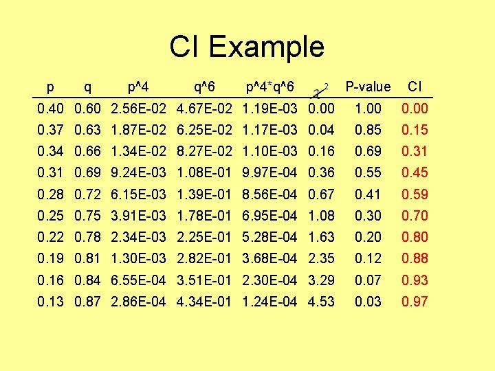
CI Example p q p^4 q^6 p^4*q^6 P-value CI 0. 40 0. 60 2. 56 E-02 4. 67 E-02 1. 19 E-03 0. 00 1. 00 0. 37 0. 63 1. 87 E-02 6. 25 E-02 1. 17 E-03 0. 04 0. 85 0. 15 0. 34 0. 66 1. 34 E-02 8. 27 E-02 1. 10 E-03 0. 16 0. 69 0. 31 0. 69 9. 24 E-03 1. 08 E-01 9. 97 E-04 0. 36 0. 55 0. 45 0. 28 0. 72 6. 15 E-03 1. 39 E-01 8. 56 E-04 0. 67 0. 41 0. 59 0. 25 0. 75 3. 91 E-03 1. 78 E-01 6. 95 E-04 1. 08 0. 30 0. 70 0. 22 0. 78 2. 34 E-03 2. 25 E-01 5. 28 E-04 1. 63 0. 20 0. 80 0. 19 0. 81 1. 30 E-03 2. 82 E-01 3. 68 E-04 2. 35 0. 12 0. 88 0. 16 0. 84 6. 55 E-04 3. 51 E-01 2. 30 E-04 3. 29 0. 07 0. 93 0. 13 0. 87 2. 86 E-04 4. 34 E-01 1. 24 E-04 4. 53 0. 03 0. 97 2
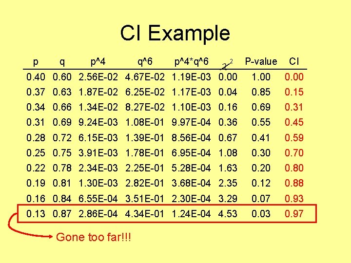
CI Example p q p^4 P-value CI 0. 40 0. 60 2. 56 E-02 4. 67 E-02 1. 19 E-03 0. 00 1. 00 0. 37 0. 63 1. 87 E-02 6. 25 E-02 1. 17 E-03 0. 04 0. 85 0. 15 0. 34 0. 66 1. 34 E-02 8. 27 E-02 1. 10 E-03 0. 16 0. 69 0. 31 0. 69 9. 24 E-03 1. 08 E-01 9. 97 E-04 0. 36 0. 55 0. 45 0. 28 0. 72 6. 15 E-03 1. 39 E-01 8. 56 E-04 0. 67 0. 41 0. 59 0. 25 0. 75 3. 91 E-03 1. 78 E-01 6. 95 E-04 1. 08 0. 30 0. 70 0. 22 0. 78 2. 34 E-03 2. 25 E-01 5. 28 E-04 1. 63 0. 20 0. 80 0. 19 0. 81 1. 30 E-03 2. 82 E-01 3. 68 E-04 2. 35 0. 12 0. 88 0. 16 0. 84 6. 55 E-04 3. 51 E-01 2. 30 E-04 3. 29 0. 07 0. 93 0. 13 0. 87 2. 86 E-04 4. 34 E-01 1. 24 E-04 4. 53 0. 03 0. 97 Gone too far!!! q^6 p^4*q^6 2
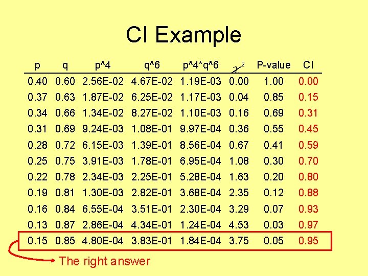
CI Example p q p^4 q^6 P-value CI 0. 40 0. 60 2. 56 E-02 4. 67 E-02 1. 19 E-03 0. 00 1. 00 0. 37 0. 63 1. 87 E-02 6. 25 E-02 1. 17 E-03 0. 04 0. 85 0. 15 0. 34 0. 66 1. 34 E-02 8. 27 E-02 1. 10 E-03 0. 16 0. 69 0. 31 0. 69 9. 24 E-03 1. 08 E-01 9. 97 E-04 0. 36 0. 55 0. 45 0. 28 0. 72 6. 15 E-03 1. 39 E-01 8. 56 E-04 0. 67 0. 41 0. 59 0. 25 0. 75 3. 91 E-03 1. 78 E-01 6. 95 E-04 1. 08 0. 30 0. 70 0. 22 0. 78 2. 34 E-03 2. 25 E-01 5. 28 E-04 1. 63 0. 20 0. 80 0. 19 0. 81 1. 30 E-03 2. 82 E-01 3. 68 E-04 2. 35 0. 12 0. 88 0. 16 0. 84 6. 55 E-04 3. 51 E-01 2. 30 E-04 3. 29 0. 07 0. 93 0. 13 0. 87 2. 86 E-04 4. 34 E-01 1. 24 E-04 4. 53 0. 03 0. 97 0. 15 0. 85 4. 80 E-04 3. 83 E-01 1. 84 E-04 3. 75 0. 05 0. 95 The right answer p^4*q^6 2

CI Caveat • Sometimes CIs are unbalanced, with one bound being much further from the estimate than the other • Don’t worry about this, as it indicates an unbalanced likelihood surface
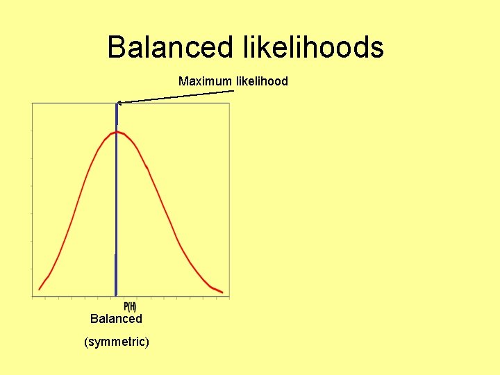
Balanced likelihoods Maximum likelihood Balanced (symmetric)
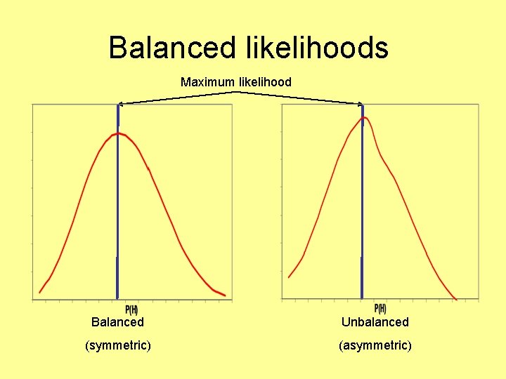
Balanced likelihoods Maximum likelihood Balanced Unbalanced (symmetric) (asymmetric)
Major recap • • Should understand what likelihood is How to calculate a likelihood How to test for significance in likelihood How to determine confidence intervals
Couple of thoughts on likelihood • Maximum likelihood is a framework which can implemented for any problem • Fundamental to likelihood is the expression of probability • One could use likelihood in the context of linear regression, instead of χ2 for testing
Maximum likelihood for continuous data • When the data of interest are continuous we must use a different form of the likelihood equation • We can estimate the mean and the variance and covariance structure • From this we define the SEMs we’ve seen
Maximum likelihood for continuous data • We assume multivariate normality (MVN): • The MVN distribution is characterized by: – 2 means, 2 variances, and 1 covariance – The nature of the covariance is as important as the 2 variances – Univariate normality for each trait is necessary but not sufficient for MVN

Picture of MVN

Ugliest formula

Ugliest formula It’s not really necessary to understand this equation. We’ll go through the important constituent parts.

Ugliest formula 2π the constant

Ugliest formula The number of means/variables

Ugliest formula The variance covariance matrix

Ugliest formula Each individual score vector

Ugliest formula Vector of means
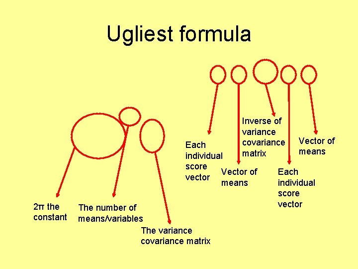
Ugliest formula Inverse of variance covariance matrix Each individual score Vector of vector means 2π the constant The number of means/variables The variance covariance matrix Vector of means Each individual score vector
Likelihood in practice • In SEM we estimate parameters from our statistics e. g.
Likelihood in practice • In SEM we estimate parameters from our statistics e. g. • A univariate example
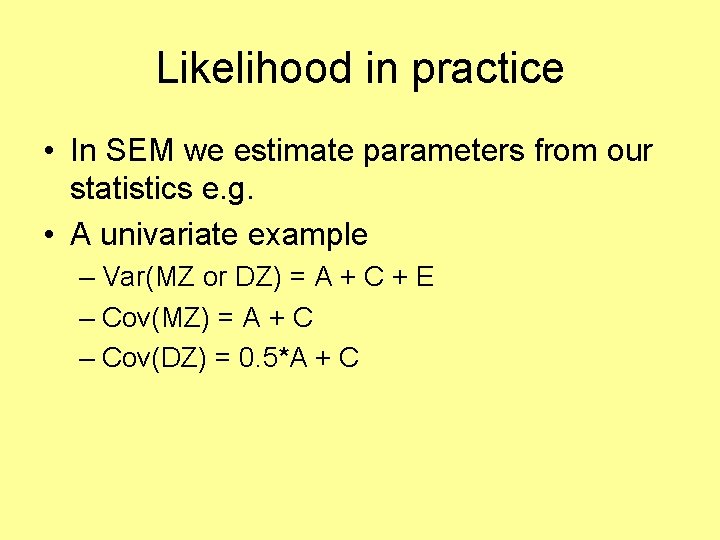
Likelihood in practice • In SEM we estimate parameters from our statistics e. g. • A univariate example – Var(MZ or DZ) = A + C + E – Cov(MZ) = A + C – Cov(DZ) = 0. 5*A + C
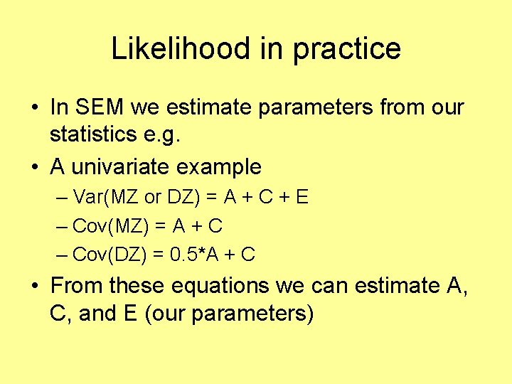
Likelihood in practice • In SEM we estimate parameters from our statistics e. g. • A univariate example – Var(MZ or DZ) = A + C + E – Cov(MZ) = A + C – Cov(DZ) = 0. 5*A + C • From these equations we can estimate A, C, and E (our parameters)
Testing parameters • From the ACE example, let’s drop A, so:
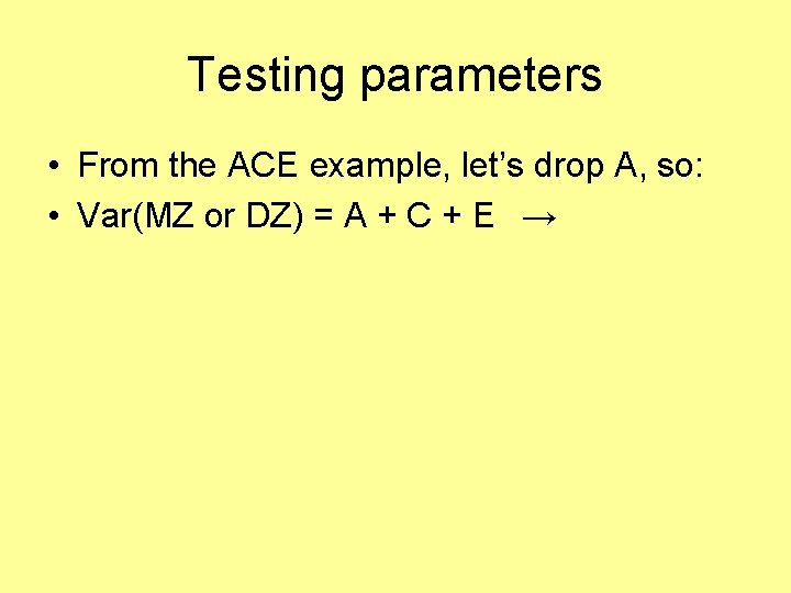
Testing parameters • From the ACE example, let’s drop A, so: • Var(MZ or DZ) = A + C + E →
Testing parameters • From the ACE example, let’s drop A, so: • Var(MZ or DZ) = A + C + E → C + E
Testing parameters • From the ACE example, let’s drop A, so: • Var(MZ or DZ) = A + C + E → C + E • Cov(MZ) = A + C → C
Testing parameters • • From the ACE example, let’s drop A, so: Var(MZ or DZ) = A + C + E → C + E Cov(MZ) = A + C → C Cov(DZ) = 0. 5*A + C → C
Testing parameters • • • From the ACE example, let’s drop A, so: Var(MZ or DZ) = A + C + E → C + E Cov(MZ) = A + C → C Cov(DZ) = 0. 5*A + C → C Effectively this is a test of what?
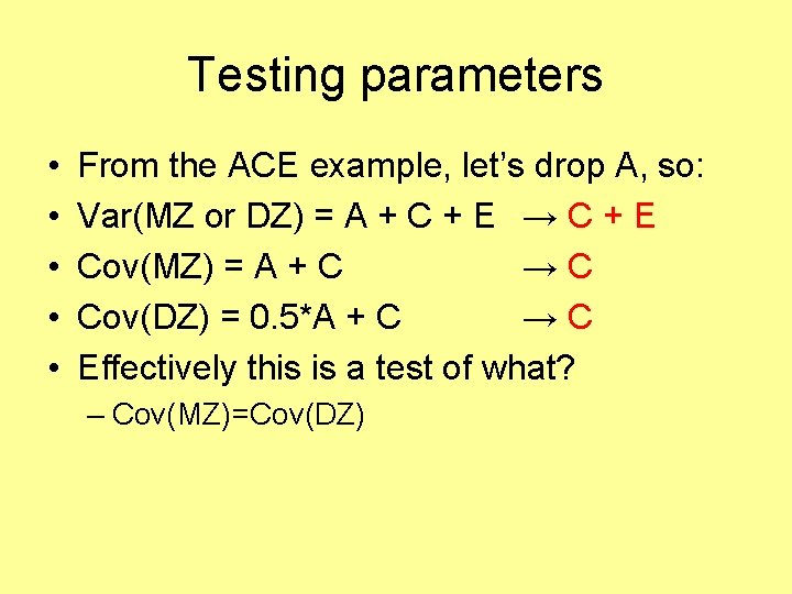
Testing parameters • • • From the ACE example, let’s drop A, so: Var(MZ or DZ) = A + C + E → C + E Cov(MZ) = A + C → C Cov(DZ) = 0. 5*A + C → C Effectively this is a test of what? – Cov(MZ)=Cov(DZ)
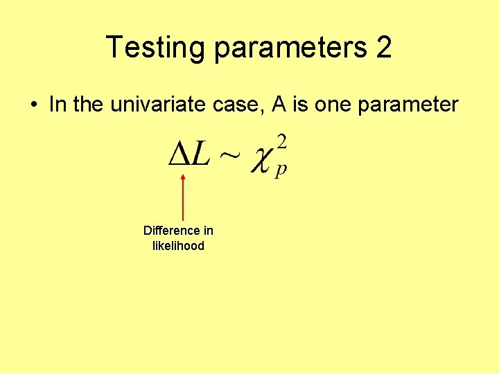
Testing parameters 2 • In the univariate case, A is one parameter Difference in likelihood
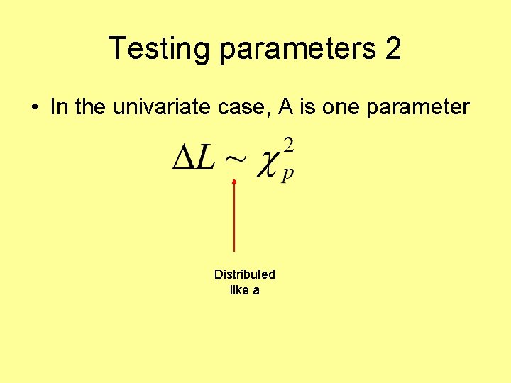
Testing parameters 2 • In the univariate case, A is one parameter Distributed like a
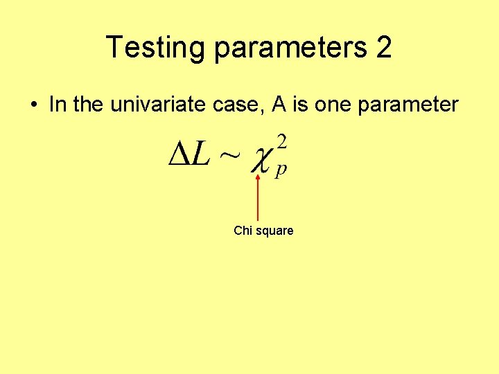
Testing parameters 2 • In the univariate case, A is one parameter Chi square
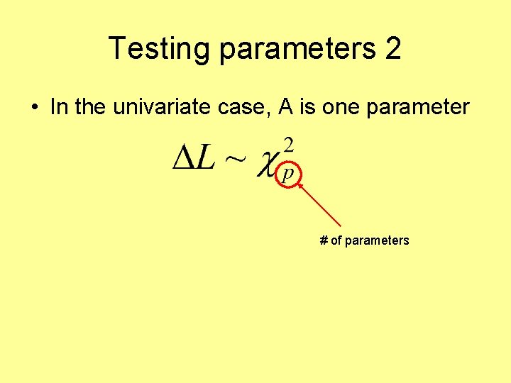
Testing parameters 2 • In the univariate case, A is one parameter # of parameters
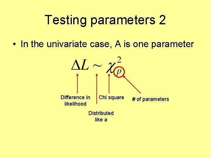
Testing parameters 2 • In the univariate case, A is one parameter Difference in likelihood Chi square Distributed like a # of parameters
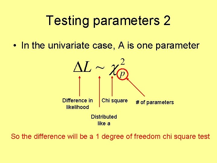
Testing parameters 2 • In the univariate case, A is one parameter Difference in likelihood Chi square # of parameters Distributed like a So the difference will be a 1 degree of freedom chi square test
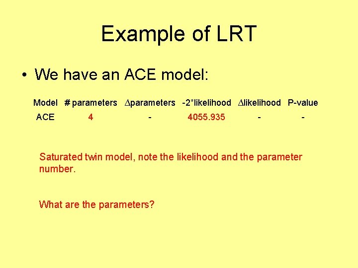
Example of LRT • We have an ACE model: Model # parameters ∆parameters -2*likelihood ∆likelihood P-value ACE 4 - 4055. 935 - - Saturated twin model, note the likelihood and the parameter number. What are the parameters?
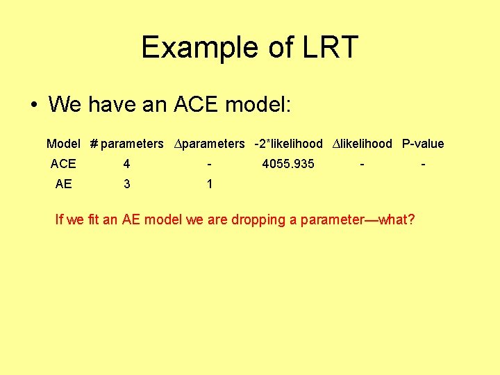
Example of LRT • We have an ACE model: Model # parameters ∆parameters -2*likelihood ∆likelihood P-value ACE 4 - AE 3 1 4055. 935 - If we fit an AE model we are dropping a parameter—what? -
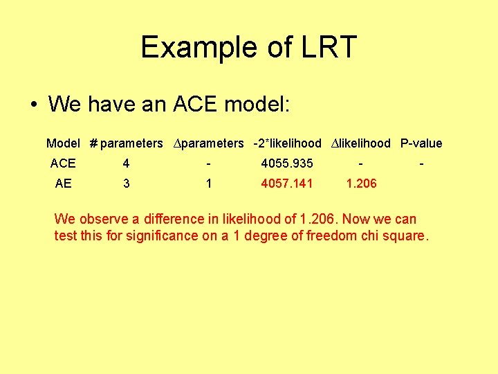
Example of LRT • We have an ACE model: Model # parameters ∆parameters -2*likelihood ∆likelihood P-value ACE 4 - 4055. 935 - AE 3 1 4057. 141 1. 206 - We observe a difference in likelihood of 1. 206. Now we can test this for significance on a 1 degree of freedom chi square.
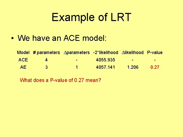
Example of LRT • We have an ACE model: Model # parameters ∆parameters -2*likelihood ∆likelihood P-value ACE 4 - 4055. 935 - - AE 3 1 4057. 141 1. 206 0. 27 What does a P-value of 0. 27 mean?
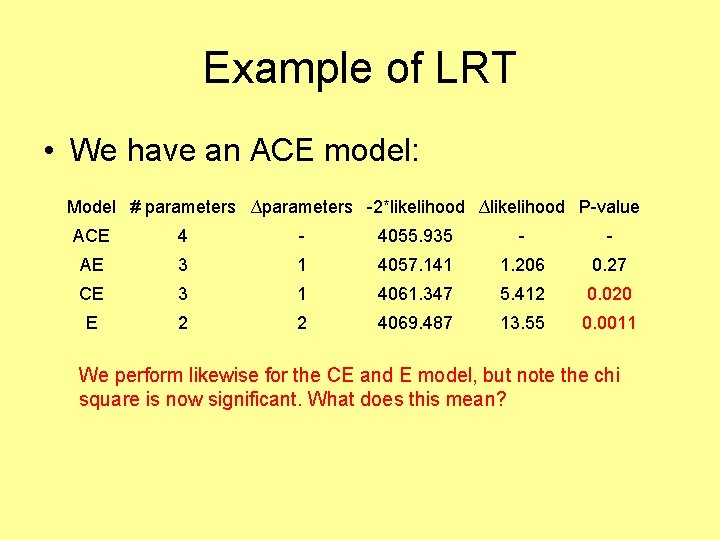
Example of LRT • We have an ACE model: Model # parameters ∆parameters -2*likelihood ∆likelihood P-value ACE 4 - 4055. 935 - - AE 3 1 4057. 141 1. 206 0. 27 CE 3 1 4061. 347 5. 412 0. 020 E 2 2 4069. 487 13. 55 0. 0011 We perform likewise for the CE and E model, but note the chi square is now significant. What does this mean?
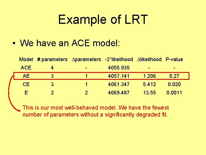
Example of LRT • We have an ACE model: Model # parameters ∆parameters -2*likelihood ∆likelihood P-value ACE 4 - 4055. 935 - - AE 3 1 4057. 141 1. 206 0. 27 CE 3 1 4061. 347 5. 412 0. 020 E 2 2 4069. 487 13. 55 0. 0011 This is our most well-behaved model. We have the fewest number of parameters without a significantly degraded fit.
Rule of parsimony • Philosophically, we favour the model with the fewest parameters that does not show a significantly worse fit
Rule of parsimony • Philosophically, we favour the model with the fewest parameters that does not show a significantly worse fit • Occam’s razor: – entia non sunt multiplicanda praeter necessitatem, or – entities should not be multiplied beyond necessity.
Rule of parsimony • Philosophically, we favour the model with the fewest parameters that does not show a significantly worse fit • Occam’s razor: – entia non sunt multiplicanda praeter necessitatem, or – entities should not be multiplied beyond necessity. • Reductionist thinking drives this as well
Nesting • Structural equation models can be nested – Effectively, this implies that you can get to a nested sub model from the original model via either dropping parameters or imposing constraints – For example, the AE, CE, and E model are nested within the ACE model, but the AE and CE models are non-nested submodels of the ACE – What is the relationship between AE and E models?
Dealing with non-nested submodels • When models are non-nested the LRT cannot be used as it requires the submodel to be nested • Fit indices such as AIC, BIC, and DIC come into play here
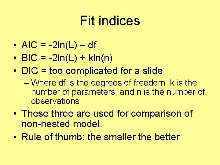
Fit indices • AIC = -2 ln(L) – df • BIC = -2 ln(L) + kln(n) • DIC = too complicated for a slide – Where df is the degrees of freedom, k is the number of parameters, and n is the number of observations • These three are used for comparison of non-nested model. • Rule of thumb: the smaller the better
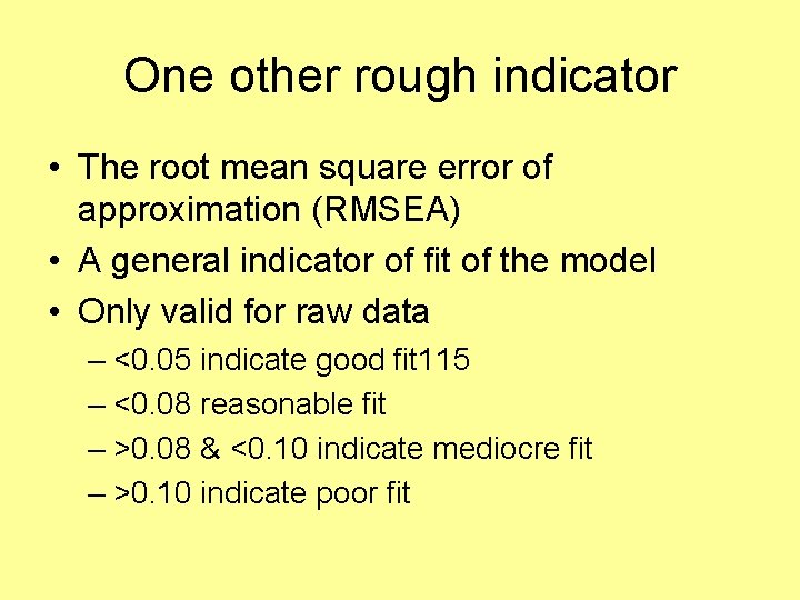
One other rough indicator • The root mean square error of approximation (RMSEA) • A general indicator of fit of the model • Only valid for raw data – <0. 05 indicate good fit 115 – <0. 08 reasonable fit – >0. 08 & <0. 10 indicate mediocre fit – >0. 10 indicate poor fit
References: • Bollen, K. A. (1989). Structural equations with latent variables. Wiley Interscience. • Browne, M. W. & Cudeck, R. (1993). Alternative ways of assessing model fit. In K. A. Bollen & J. S. Long (Eds. ), Testing structural equation models (pp. 136 -162). Newbury Park, CA: Sage. • Mac. Callum, R. C. , Browne, M. W. , Sugawara, H. M. (1996). Power analysis and determination of sample size for covariance structure modeling. Psychological Methods, 1, 130 -149. • Markon, K. E. , and Krueger, R. F. (2004). An Empirical Comparison of Information-Theoretic Selection Criteria for Multivariate Behavior Genetic Models. Behavior Genetics, 34, 593 -610 Mx Scripts Library hosted at Genom. EUtwin very useful for scripts and information http: //www. psy. vu. nl/mxbib/. See TIPS and FAQ sections. • Neale MC, Boker SM, Xie G, Maes HH (2003). Mx: Statistical Modeling. VCU Box 900126, Richmond, VA 23298: Department of Psychiatry. 6 th Edition. • Raftery, A. E. (1995). Bayesian model selection in social research. Sociological Methodology (ed. Peter V. Marsden), Oxford, U. K. : Blackwells, pp. 111 -196.
- Slides: 116