Max Min Fairness How define fairness Any session

Max Min Fairness • How define fairness? • “Any session is entitled to as much network use as is any other” • …. unless some sessions can use more without hurting others • Other definitions – Network usage depends on the resource consumption by the session – Pay/bid for what you use

A Simple Example • Max-min allocation: 1/3, 2/3

How to Calculate Max Min Flow Share Fluid model: 1. Increase the flow until some pipe fills-up. 2. Fix the bandwidth of the bottleneck flows 3. Continue with the unfixed flows Can be done efficiently by calculating the bottleneck link at step 1

Buffer management and admission control Simplest admission policy: • Accept packets until buffer is full (tail drop) We already saw: • Tail drop is not kind to TCP flows • RED can be used to avoid tail drop

Reminder: Hallelujah for RED • Random early detection (RED) makes three improvements • Metric is moving average of queue lengths – small bursts pass through unharmed – only affects sustained overloads • Packet drop probability is a function of mean queue length – prevents severe reaction to mild overload • Can mark packets instead of dropping them ECN – allows sources to detect network state without losses • RED improves performance of a network of cooperating TCP sources • No bias against bursty sources • Controls queue length regardless of endpoint cooperation

How does it work? Drop probability 1 RED gentle RED max-p Max-thresh 2*Max-thresh Average Q size

So problem is solved? • Fairly easy to implement in hardware! • Can work in wire-speed! • All we need to do is set the parameters…. . right • Turns out there is no universal good set of parameters • Some studies show RED has NO advantage over tail drop. WHY?

parameters avg. Q= (1 -wq)avg. Q+wqq Floyd-Jacobson: • Wq: 0. 002, not less than 0. 001 • max_p: 1/50, • max_th: at least twice min_th • max_th-min_th larger than the q increase in RTT • Future work …. .

So does it help us to surf? Tuning RED for Web Traffic, Christiansen et al. , SIGCOMM 2000 (1) compared to a (properly configured) FIFO queue, RED has a minimal effect on HTTP response times for offered loads up to 90% of link capacity, (2) response times at loads in this range are not substantially effected by RED control parameters, (3) between 90% and 100% load, RED can be carefully tuned to yield performance somewhat superior to FIFO, however, response times are quite sensitive to the actual RED parameter values selected, and (4) in such congested networks, RED parameters that provide the best link utilization produce poorer response times.

SPRINT study (Diot et al. ) • A parallel study, presented at NANOG 2000 • Testbed – with CISCO routers (7500) – with Dummynet • used “recommended” RED and GRED parameters • Heterogeneous delays (120 to 180 ms)

Traffic characteristics • 16 to 256 TCP connections sharing the bottleneck. • Experimental traffic generated by Chariot – long-lived TCP connections. – more “realistic” traffic mix: • 90% short lived TCP connections (up to 20 packets) • 10 % long lived TCP connections – 1 Mbps UDP in both cases

Testbed (CISCO routers) 7500 10 Megs 7500

Testbed (Dummynet) 10 Megs 7500 100 Megs Dummy net 7500

What is Dummynet? application dummynet network

Metrics observed • • Aggregate goodput through a router TCP and UDP loss rate Consecutive losses Queuing behavior

Aggregate goodput (long-lived TCP)

256 short and long lived TCP connections

Consecutive packet losses (long lived)

…if we use “optimal” RED parameters

Consecutive packet losses (realistic traffic mix)

Queuing behavior (256 long lived connections)

Queuing behavior (256 connections, realistic mix)

Diot’s summary • No significant difference on goodput, TCP losses and UDP losses. • On consecutive losses, clear advantage to GRED and GRED-I. • “gentle” modification solves many RED problems. • Oscillations: no clear winner. Traffic seems to be the determining factor.

From the ISP standpoint. . . • Not clear there is an advantage in deploying RED, GRED, or GRED-I. • Maybe GRED-I is an option if one can find a “universal” exponential dropping function. • ECN will work with any scheme. • Not clear the solution is in the AQM space.

GRED-I with exponential dropping function 1 buffer size

Deficit Round Robin (DRR) • A modification to WRR to overcome different packet sizes. • No need to know the average packet size. • Each Q is associated with a deficit counter. – Initiated to 0. – Holds the Q’s deficit in service

DRR Algorithm: • If size(HOL packet) ≤ quota + deficit – Send packet – deficit+quota-(packet size) • Else – Don’t send packet – deficit+quota

About Fair Queuing. . . • Not only feasible … easy at the edges! – www. agere. com (an example) – vendors support from 64 k to 200 k flows • Really fair – everybody gets what he/she paid for • local signaling (end host to CPE)

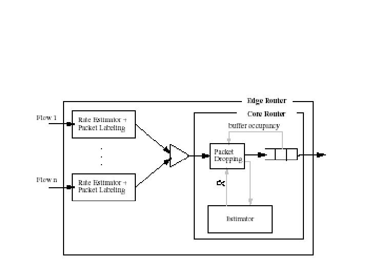
fair queueing at the edge Core-stateless fair queueing • WFQ is hard to do at the core • Edge routers estimate rate and label packets • Core routers maintain FIFO queues and drop based on label

CSFQ summary • Better than FIFO and RED • Similar to FRED • Not as good as DRR

Rainbow fair queueing • Similar to CSFQ • Have similar performance as CSFQ • Enable applications to mark packets and achieve better goodput

Rainbow Fair Queueing (RFQ) • Example – A: 10 Kbps B: 6 Kbps C: 8 Kbps – Each layer: 2 Kbps

RFQ: basic mechanism (1) the estimation of the flow arrival rate at the edge routers (2) the selection of the rates for each color (3) the assignment of colors to packets (4) the core router algorithm

Rainbow Fair Queueing (RFQ) (1) the estimation of the flow arrival rate at the edge routers • • • rinew: arrival rate tik: arrival time of flow I lik: length of the kth packet of flow I K: a constant Tik = tik – tik-1

Rainbow Fair Queueing (RFQ) (2) the selection of the rates for each color • • ci: i color average rate of packets N: total number of colors and multiple of b a, b: determine the block structure P: the maximum flow rate in the network

Rainbow Fair Queueing (RFQ): Example • N=8 a=b=2 c 0 c 1 c 2 c 3 c 4 c 5 c 6 c 7 P/16 P/8 P/4

Rainbow Fair Queueing (RFQ) (3) the assignment of colors to packets – Suppose the current estimate of the flow arrival rate is r, and j is the smallest value satisfying. – Then the current packet is assigned color with probability.

(4) the core router algo. • Conditions to decrease color: – – q threshold Flow bw Positive gradient Hold you horses • Conditions to increase color – Time – Flow below service rate

Rainbow Fair Queueing (RFQ) • Weighted RFQ – wi: weight for flow i – c j = w ic j

Simulations: A single congested link

Fairness: flow i sends at 0. 313 i

Throughput: TCP flow

Throughput: UDP flows

Control Responsiveness 10 Mbps: 8 x 1 M 7 x 1 M+8 M

Simulations: Performance Effects of Buffer Size

Simulations: TCP Performance Under Various round Trip Delay