Matrix Operator scaling and their many applications Avi

![PMs & symbolic matrices U V G [Edmonds‘ 67] 1 1 1 x 12 PMs & symbolic matrices U V G [Edmonds‘ 67] 1 1 1 x 12](https://slidetodoc.com/presentation_image_h2/febaa924d31d0c9e9a8cd005dd33e4af/image-5.jpg)
![Matrix scaling algorithm [Sinkhorn’ 64, LSW’ 01, GY’ 03] A non-negative matrix. Try making Matrix scaling algorithm [Sinkhorn’ 64, LSW’ 01, GY’ 03] A non-negative matrix. Try making](https://slidetodoc.com/presentation_image_h2/febaa924d31d0c9e9a8cd005dd33e4af/image-8.jpg)
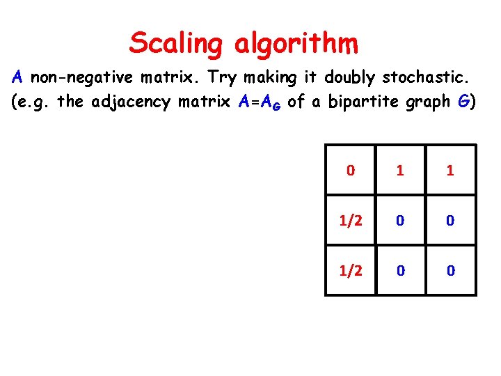
![Scaling algorithm [LSW ‘ 01] A non-negative matrix. Try making it doubly stochastic. (e. Scaling algorithm [LSW ‘ 01] A non-negative matrix. Try making it doubly stochastic. (e.](https://slidetodoc.com/presentation_image_h2/febaa924d31d0c9e9a8cd005dd33e4af/image-13.jpg)
![Scaling algorithm [LSW ‘ 01] A non-negative matrix. Try making it doubly stochastic. (e. Scaling algorithm [LSW ‘ 01] A non-negative matrix. Try making it doubly stochastic. (e.](https://slidetodoc.com/presentation_image_h2/febaa924d31d0c9e9a8cd005dd33e4af/image-14.jpg)
![Scaling algorithm [LSW ‘ 01] A non-negative matrix. Try making it doubly stochastic. (e. Scaling algorithm [LSW ‘ 01] A non-negative matrix. Try making it doubly stochastic. (e.](https://slidetodoc.com/presentation_image_h2/febaa924d31d0c9e9a8cd005dd33e4af/image-15.jpg)
![Scaling algorithm [LSW ‘ 01] A non-negative matrix. Try making it doubly stochastic. (e. Scaling algorithm [LSW ‘ 01] A non-negative matrix. Try making it doubly stochastic. (e.](https://slidetodoc.com/presentation_image_h2/febaa924d31d0c9e9a8cd005dd33e4af/image-16.jpg)
![Scaling algorithm [LSW ‘ 01] A non-negative (0, 1) matrix. “Make it doubly stochastic” Scaling algorithm [LSW ‘ 01] A non-negative (0, 1) matrix. “Make it doubly stochastic”](https://slidetodoc.com/presentation_image_h2/febaa924d31d0c9e9a8cd005dd33e4af/image-17.jpg)
![Operator scaling algorithm [Gurvits ’ 04, GGOW’ 15] L=(A 1, A 2, …, Am). Operator scaling algorithm [Gurvits ’ 04, GGOW’ 15] L=(A 1, A 2, …, Am).](https://slidetodoc.com/presentation_image_h2/febaa924d31d0c9e9a8cd005dd33e4af/image-18.jpg)
![Quantum information theory Completely positive maps [Gurvits ’ 04] L=(A 1, A 2, …, Quantum information theory Completely positive maps [Gurvits ’ 04] L=(A 1, A 2, …,](https://slidetodoc.com/presentation_image_h2/febaa924d31d0c9e9a8cd005dd33e4af/image-23.jpg)
![Analysis (and beyond!) Brascamp-Lieb Inequalities [BL’ 76, Lieb’ 90] B = (B 1, B Analysis (and beyond!) Brascamp-Lieb Inequalities [BL’ 76, Lieb’ 90] B = (B 1, B](https://slidetodoc.com/presentation_image_h2/febaa924d31d0c9e9a8cd005dd33e4af/image-24.jpg)
- Slides: 27

Matrix & Operator scaling and their many applications Avi Wigderson IAS, Princeton

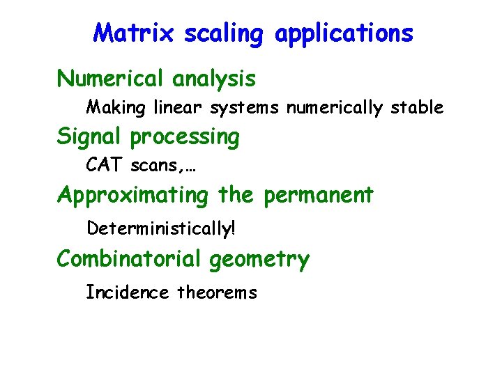
Matrix scaling applications Numerical analysis Making linear systems numerically stable Signal processing CAT scans, … Approximating the permanent Deterministically! Combinatorial geometry Incidence theorems

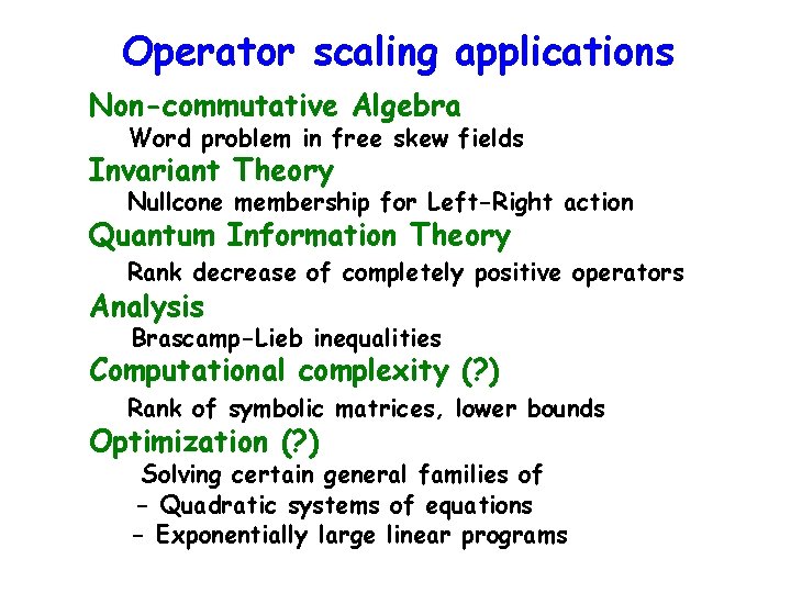
Operator scaling applications Non-commutative Algebra Word problem in free skew fields Invariant Theory Nullcone membership for Left-Right action Quantum Information Theory Rank decrease of completely positive operators Analysis Brascamp-Lieb inequalities Computational complexity (? ) Rank of symbolic matrices, lower bounds Optimization (? ) Solving certain general families of - Quadratic systems of equations - Exponentially large linear programs

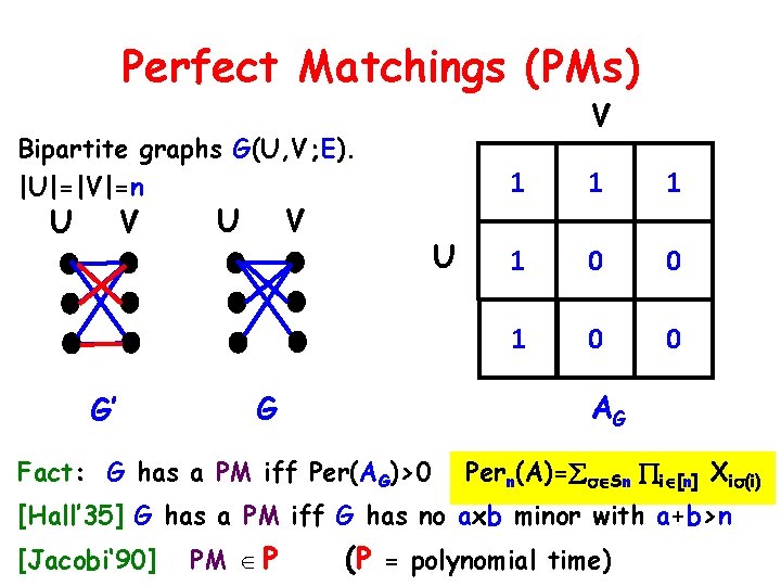
Perfect Matchings (PMs) V Bipartite graphs G(U, V; E). |U|=|V|=n U V G’ U V U 1 1 0 0 AG G Fact: G has a PM iff Per(AG)>0 Pern(A)= Sn i [n] Xi (i) [Hall’ 35] G has a PM iff G has no axb minor with a+b>n [Jacobi‘ 90] PM P (P = polynomial time)
![PMs symbolic matrices U V G Edmonds 67 1 1 1 x 12 PMs & symbolic matrices U V G [Edmonds‘ 67] 1 1 1 x 12](https://slidetodoc.com/presentation_image_h2/febaa924d31d0c9e9a8cd005dd33e4af/image-5.jpg)
PMs & symbolic matrices U V G [Edmonds‘ 67] 1 1 1 x 12 x 13 1 0 0 x 21 0 0 x 31 0 0 AG AG(X) [Edmonds ‘ 67] G has a PM iff Det(AG(X)) 0 ( P)

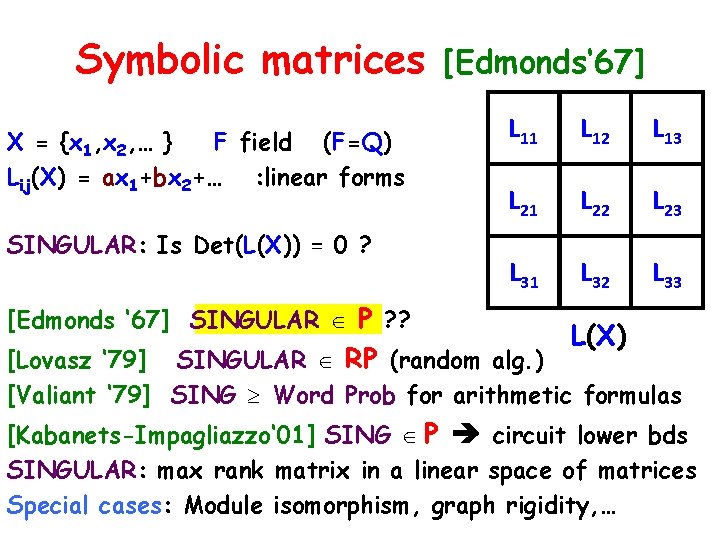
Symbolic matrices X = {x 1, x 2, … } F field (F=Q) Lij(X) = ax 1+bx 2+… : linear forms SINGULAR: Is Det(L(X)) = 0 ? [Edmonds ‘ 67] SINGULAR P ? ? [Edmonds‘ 67] L 11 L 12 L 13 L 21 L 22 L 23 L 31 L 32 L 33 L(X) [Lovasz ‘ 79] SINGULAR RP (random alg. ) [Valiant ‘ 79] SING Word Prob for arithmetic formulas [Kabanets-Impagliazzo‘ 01] SING P circuit lower bds SINGULAR: max rank matrix in a linear space of matrices Special cases: Module isomorphism, graph rigidity, …

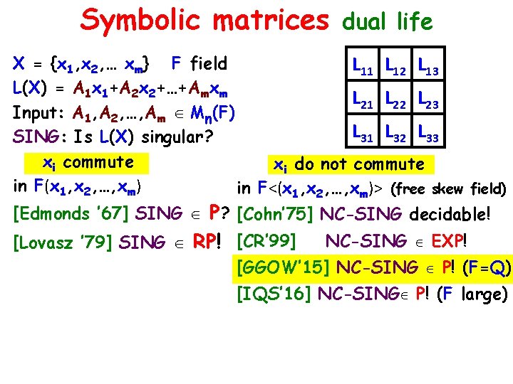
Symbolic matrices dual life X = {x 1, x 2, … xm} F field L 11 L 12 L 13 L(X) = A 1 x 1+A 2 x 2+…+Amxm L 21 L 22 L 23 Input: A 1, A 2, …, Am Mn(F) L 31 L 32 L 33 SING: Is L(X) singular? xi commute xi do not commute in F(x 1, x 2, …, xm) in F<(x 1, x 2, …, xm)> (free skew field) [Edmonds ’ 67] SING P? [Cohn’ 75] NC-SING decidable! NC-SING EXP! [Lovasz ’ 79] SING RP! [CR’ 99] [GGOW’ 15] NC-SING P! (F=Q) [IQS’ 16] NC-SING P! (F large)
![Matrix scaling algorithm Sinkhorn 64 LSW 01 GY 03 A nonnegative matrix Try making Matrix scaling algorithm [Sinkhorn’ 64, LSW’ 01, GY’ 03] A non-negative matrix. Try making](https://slidetodoc.com/presentation_image_h2/febaa924d31d0c9e9a8cd005dd33e4af/image-8.jpg)
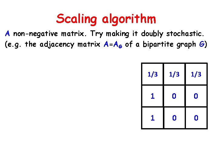
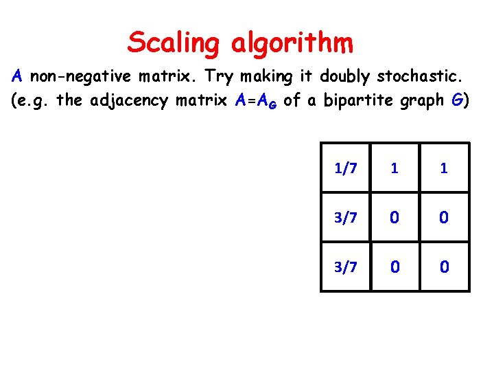
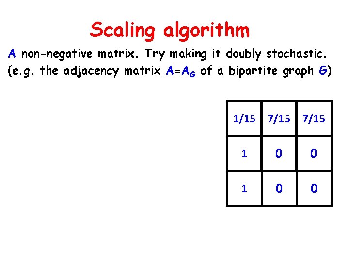
Matrix scaling algorithm [Sinkhorn’ 64, LSW’ 01, GY’ 03] A non-negative matrix. Try making it doubly stochastic. (e. g. the adjacency matrix A=AG of a bipartite graph G) Allowed: 1 1 1 Multiply rows & columns by scalars 1 0 0 Find (if exists? ) R, C diagonal s. t. RAC has row-sums & col-sums =1 1 1 0 0

Scaling algorithm A non-negative matrix. Try making it doubly stochastic. (e. g. the adjacency matrix A=AG of a bipartite graph G) 1/3 1/3 1 0 0

Scaling algorithm A non-negative matrix. Try making it doubly stochastic. (e. g. the adjacency matrix A=AG of a bipartite graph G) 1/7 1 1 3/7 0 0

Scaling algorithm A non-negative matrix. Try making it doubly stochastic. (e. g. the adjacency matrix A=AG of a bipartite graph G) 1/15 7/15 1 0 0

Scaling algorithm A non-negative matrix. Try making it doubly stochastic. (e. g. the adjacency matrix A=AG of a bipartite graph G) 0 1 1 1/2 0 0
![Scaling algorithm LSW 01 A nonnegative matrix Try making it doubly stochastic e Scaling algorithm [LSW ‘ 01] A non-negative matrix. Try making it doubly stochastic. (e.](https://slidetodoc.com/presentation_image_h2/febaa924d31d0c9e9a8cd005dd33e4af/image-13.jpg)
Scaling algorithm [LSW ‘ 01] A non-negative matrix. Try making it doubly stochastic. (e. g. the adjacency matrix A=AG of a bipartite graph G) R(A) = diag(row sums)-1 C(A) = diag(column sums)-1 Repeat n 3 times: Normalize rows A �R(A) A Normalize cols A �A C(A) 1 1 1 0 0
![Scaling algorithm LSW 01 A nonnegative matrix Try making it doubly stochastic e Scaling algorithm [LSW ‘ 01] A non-negative matrix. Try making it doubly stochastic. (e.](https://slidetodoc.com/presentation_image_h2/febaa924d31d0c9e9a8cd005dd33e4af/image-14.jpg)
Scaling algorithm [LSW ‘ 01] A non-negative matrix. Try making it doubly stochastic. (e. g. the adjacency matrix A=AG of a bipartite graph G) R(A) = diag(row sums)-1 C(A) = diag(column sums)-1 Repeat n 3 times: Normalize rows A �R(A) A Normalize cols A �A C(A) 1/3 1/3 1/2 0 1 0 0
![Scaling algorithm LSW 01 A nonnegative matrix Try making it doubly stochastic e Scaling algorithm [LSW ‘ 01] A non-negative matrix. Try making it doubly stochastic. (e.](https://slidetodoc.com/presentation_image_h2/febaa924d31d0c9e9a8cd005dd33e4af/image-15.jpg)
Scaling algorithm [LSW ‘ 01] A non-negative matrix. Try making it doubly stochastic. (e. g. the adjacency matrix A=AG of a bipartite graph G) R(A) = diag(row sums)-1 C(A) = diag(column sums)-1 Repeat n 3 times: Normalize rows A �R(A) A Normalize cols A �A C(A) 2/11 2/5 1 3/11 3/5 0 6/11 0 0
![Scaling algorithm LSW 01 A nonnegative matrix Try making it doubly stochastic e Scaling algorithm [LSW ‘ 01] A non-negative matrix. Try making it doubly stochastic. (e.](https://slidetodoc.com/presentation_image_h2/febaa924d31d0c9e9a8cd005dd33e4af/image-16.jpg)
Scaling algorithm [LSW ‘ 01] A non-negative matrix. Try making it doubly stochastic. (e. g. the adjacency matrix A=AG of a bipartite graph G) R(A) = diag(row sums)-1 C(A) = diag(column sums)-1 Repeat n 3 times: Normalize rows A �R(A) A Normalize cols A �A C(A) 10/87 22/87 55/87 15/48 33/48 1 0 0 0
![Scaling algorithm LSW 01 A nonnegative 0 1 matrix Make it doubly stochastic Scaling algorithm [LSW ‘ 01] A non-negative (0, 1) matrix. “Make it doubly stochastic”](https://slidetodoc.com/presentation_image_h2/febaa924d31d0c9e9a8cd005dd33e4af/image-17.jpg)
Scaling algorithm [LSW ‘ 01] A non-negative (0, 1) matrix. “Make it doubly stochastic” (e. g. the adjacency matrix A=AG of a bipartite graph G) R(A) = diag(row sums)-1 C(A) = diag(column sums)-1 Repeat n 3 times: Normalize rows A �R(A) A Normalize cols A �A C(A) (C(A)=I) Test if R(A) I (up to 1/n) Yes: Per(A) > 0. No: Per(A) = 0. Analysis: - 0 0 1 0 1 0 0 Initially Per(A) > exp(-n) (easy) Per(A) grows by (1+1/n) (AMGM) Per(A) ≤ 1 |R(A)-I|< 1/n Per(A) >0 (Cauchy-Schwarz)
![Operator scaling algorithm Gurvits 04 GGOW 15 LA 1 A 2 Am Operator scaling algorithm [Gurvits ’ 04, GGOW’ 15] L=(A 1, A 2, …, Am).](https://slidetodoc.com/presentation_image_h2/febaa924d31d0c9e9a8cd005dd33e4af/image-18.jpg)
Operator scaling algorithm [Gurvits ’ 04, GGOW’ 15] L=(A 1, A 2, …, Am). Try making it “doubly stochastic” i. Ait=I i. Ait. Ai=I. Allowed: L RLC, R(L) = ( i. Ait)-1/2 C(L) = ( i. Ait. Ai)-1/2 Repeat nc times: Normalize rows L �R(L) L Normalize cols L �L C(L) Test if C(L) I (up to 1/n) Yes: L NC-nonsingular No: L NC-singular Analysis: Capacity(L) > exp(-n) Cap(A) grows by (1+1/n) Cap(A) ≤ 1 |R(L)-I|< 1/n Cap(A) 1 R, C invertible Invertible [GGOW’ 15] - NC-rank P - Computes Cap(L) & scaling factors - Alg continuous in L [G’ 04, GGOW’ 15] (AMGM) (Cauchy-Schwarz)

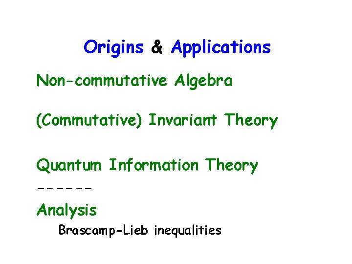
Origins & Applications Non-commutative Algebra (Commutative) Invariant Theory Quantum Information Theory -----Analysis Brascamp-Lieb inequalities

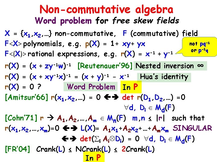
Non-commutative algebra Word problem for free skew fields X = {x 1, x 2, …} non-commutative, F (commutative) field not pq-1 F<X> polynomials, e. g. p(X) = 1+ xy+ yx -1 q or p F<(X)> rational expressions, e. g. r(X) = x-1 + y-1 r(X) = (x + zy-1 w)-1 [Reutenauer’ 96] Nested inversion ∞ r(X) = (x + xy-1 x)-1 = (x + y)-1 - x-1 Hua’s identity r(X) = 0 ? Word Problem In P [Amitsur’ 66] r(x 1, x 2, …) = 0 det r(D 1, D 2, …) =0 d, Di Md(F) [Cohn’ 71] r A 1, A 2, …, Am Mn(F) m, n ≤ |r| such that r(x 1, x 2, …, xm)=0 L(X)= A 1 x 1+A 2 x 2+…+Amxm SINGULAR det( i Ai Di) = 0 d, Di Md(F) [FR’ 04] Crank(L) ≤ NCrank(L) ≤ 2 Crank(L) In P

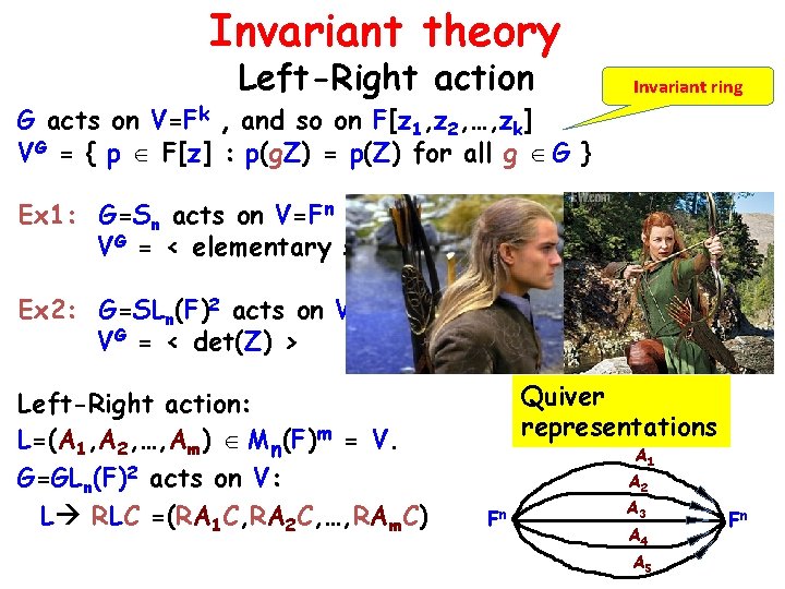
Invariant theory Left-Right action G acts on V=Fk , and so on F[z 1, z 2, …, zk] VG = { p F[z] : p(g. Z) = p(Z) for all g G } Invariant ring Ex 1: G=Sn acts on V=Fn by permuting coordinates VG = < elementary symmetric polynomials > Ex 2: G=SLn(F)2 acts on V=Mn(F) VG = < det(Z) > Left-Right action: L=(A 1, A 2, …, Am) Mn(F)m = V. G=GLn(F)2 acts on V: L RLC =(RA 1 C, RA 2 C, …, RAm. C) by Z RZC Quiver representations A 1 Fn A 2 A 3 A 4 A 5 Fn

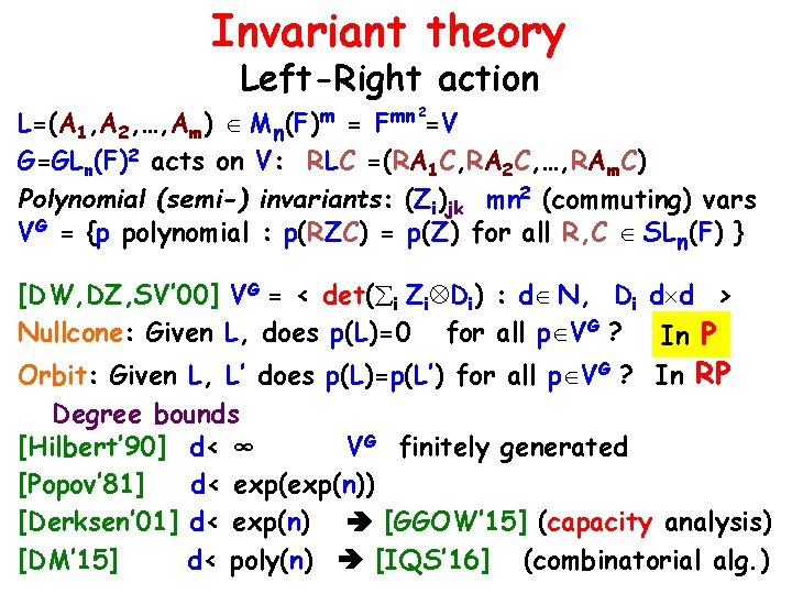
Invariant theory Left-Right action L=(A 1, A 2, …, Am) Mn(F)m = Fmn =V G=GLn(F)2 acts on V: RLC =(RA 1 C, RA 2 C, …, RAm. C) Polynomial (semi-) invariants: (Zi)jk mn 2 (commuting) vars VG = {p polynomial : p(RZC) = p(Z) for all R, C SLn(F) } 2 [DW, DZ, SV’ 00] VG = < det( i Zi Di) : d N, Di d d > Nullcone: Given L, does p(L)=0 for all p VG ? In P Orbit: Given L, L’ does p(L)=p(L’) for all p VG ? In RP Degree bounds [Hilbert’ 90] d< ∞ VG finitely generated [Popov’ 81] d< exp(n)) [Derksen’ 01] d< exp(n) [GGOW’ 15] (capacity analysis) [DM’ 15] d< poly(n) [IQS’ 16] (combinatorial alg. )
![Quantum information theory Completely positive maps Gurvits 04 LA 1 A 2 Quantum information theory Completely positive maps [Gurvits ’ 04] L=(A 1, A 2, …,](https://slidetodoc.com/presentation_image_h2/febaa924d31d0c9e9a8cd005dd33e4af/image-23.jpg)
Quantum information theory Completely positive maps [Gurvits ’ 04] L=(A 1, A 2, …, Am) Ai Mn(C) completely positive map: Quantum L(P)= i. Ai. PAit (P psd L(P) psd) breaking entanglements (noise) operator “Hall Condition” L rank-decreasing if exists P psd s. t. rk(L(P)) < rk(P) [Cohn’ 71] L rank-decreasing L NC-singular. In P Quasi. L doubly stochastic if i. Ait=I i. Ait. Ai=I convex Capacity(L) = inf { det(L(P)) / det(P) : P psd } [Gurvits] L rank-decreasing Cap(L) = 0 L doubly stochastic Cap(L) = 1 L’ = RLC Cap(L’) = Cap(L) det(R)2 det(C)2 Capacity tensorizes: Cap(A 1 D 1, …, Am Dm)=… [GGOW’ 15] Use degree bounds in capacity analysis
![Analysis and beyond BrascampLieb Inequalities BL 76 Lieb 90 B B 1 B Analysis (and beyond!) Brascamp-Lieb Inequalities [BL’ 76, Lieb’ 90] B = (B 1, B](https://slidetodoc.com/presentation_image_h2/febaa924d31d0c9e9a8cd005dd33e4af/image-24.jpg)
Analysis (and beyond!) Brascamp-Lieb Inequalities [BL’ 76, Lieb’ 90] B = (B 1, B 2, …, Bm) Bj: Rn Rnj p = (pj, p 2, …, pm) pj ≥ 0 ∫x Rn (∏j fj(Bj(x)))pj (B, p): BL data ≤ C ∏j (∫xj Rnj fj(xj))pj fixed C [0, ∞) f = (f 1, f 2, …, fm) fj: Rnj R integrable Cauchy-Schwarz, Holder Precopa-Leindler Loomis-Whitney Nelson Hypercontractive Young’s convolution Brunn-Minkowski Bennett-Nez Nonlinear BL quantitative Helly Lieb’s Non-commutative BL Barthe Reverse BL Bourgain et al Multilinear estimates, decoupling, Kakeya, restriction, Weyl sums, maximal functions, …

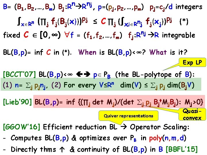
B= (B 1, B 2, …, Bm) Bj: Rn Rnj, p=(pj, p 2, …, pm) pj=cj/d integers ∫x Rn (∏j fj(Bj(x)))pj ≤ C ∏j (∫xj Rnj fj(xj))pj (*) fixed C [0, ∞) f = (f 1, f 2, …, fm) fj: Rnj R integrable BL(B, p)= inf C in (*). When is BL(B, p)<∞? What is it? Exp LP [BCCT’ 07] BL(B, p)<∞ p PB (the BL-polytope of B): (1) n= j pjnj, (2) For every V≤Rn dim(V) ≤ j pj dim(Bj. V) [Lieb’ 90] BL(B, p)= inf {(∏j det Mj)/(det j pj Bjt. Mj. Bj): Mj>0} Quiver representations Quasiconvex [GGOW’ 16] Efficient reduction BL Operator Scaling: - Computes BL(B, p) & optimizes over PB in poly(n, m, d) - Directly thms ↑ & continuity of BL(B, p) in B [BBFL’ 15]

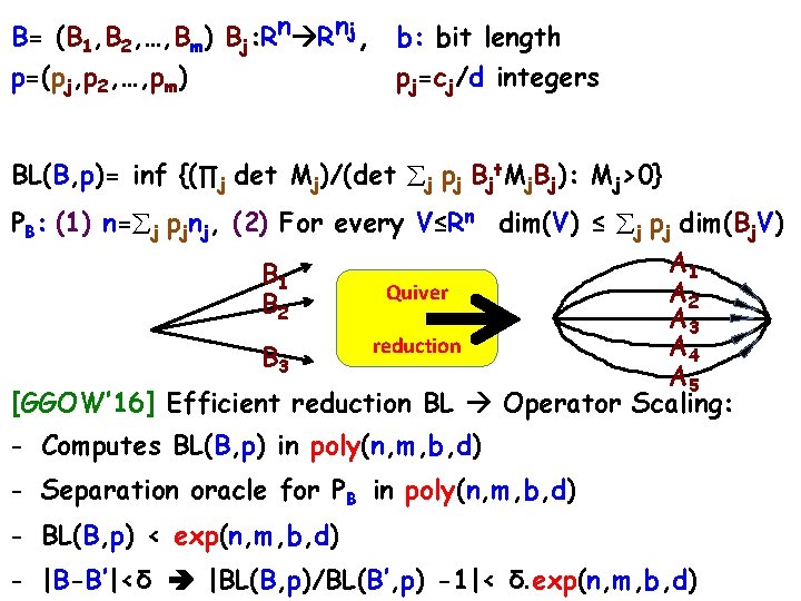
B= (B 1, B 2, …, Bm) Bj: Rn Rnj, b: bit length p=(pj, p 2, …, pm) pj=cj/d integers BL(B, p)= inf {(∏j det Mj)/(det j pj Bjt. Mj. Bj): Mj>0} PB: (1) n= j pjnj, (2) For every V≤Rn dim(V) ≤ j pj dim(Bj. V) A 1 B 1 Quiver A 2 B 2 A 3 reduction A 4 B 3 A 5 [GGOW’ 16] Efficient reduction BL Operator Scaling: - Computes BL(B, p) in poly(n, m, b, d) - Separation oracle for PB in poly(n, m, b, d) - BL(B, p) < exp(n, m, b, d) - |B-B’|<δ |BL(B, p)/BL(B’, p) -1|< δ. exp(n, m, b, d)

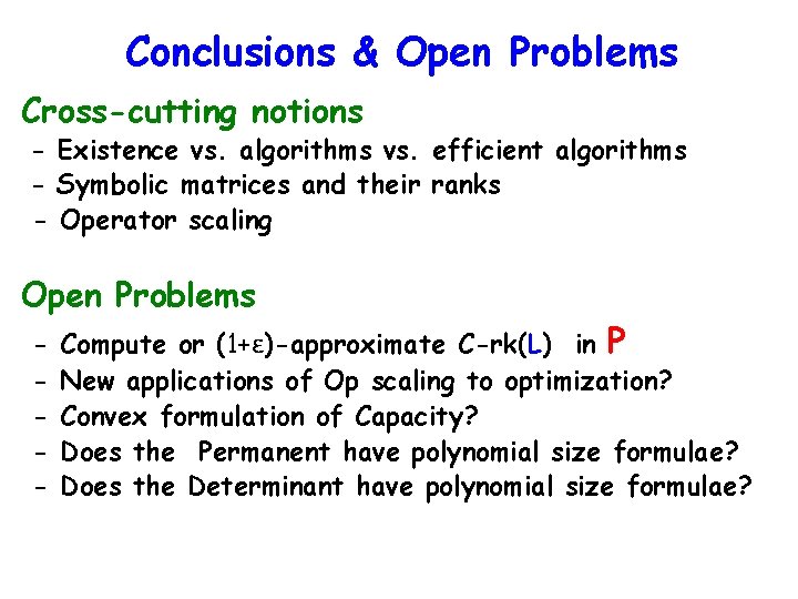
Conclusions & Open Problems Cross-cutting notions - Existence vs. algorithms vs. efficient algorithms - Symbolic matrices and their ranks - Operator scaling Open Problems - Compute or (1+ε)-approximate C-rk(L) in P New applications of Op scaling to optimization? Convex formulation of Capacity? Does the Permanent have polynomial size formulae? Does the Determinant have polynomial size formulae?