Matrix Multiplication and Graph Algorithms Uri Zwick Tel


 time.")
 …")
 2.")

 = 8 T(n/2) + O(n")
![“Master method” for recurrences [CLRS 3 rd Ed. , p. 94]](https://slidetodoc.com/presentation_image/2ead93bd2755be695e2ca87afd612657/image-8.jpg "“Master method” for recurrences [CLRS 3 rd Ed. , p. 94]")


![LUP decomposition (in pictures) [Bunch-Hopcroft (1974)] n m A = [AHU’ 74, Section 6.](https://slidetodoc.com/presentation_image/2ead93bd2755be695e2ca87afd612657/image-17.jpg "LUP decomposition (in pictures) [Bunch-Hopcroft (1974)] n m A = [AHU’ 74, Section 6.")
![LUP decomposition (in pictures) [Bunch-Hopcroft (1974)] n m/2 B m/2 C n m =m](https://slidetodoc.com/presentation_image/2ead93bd2755be695e2ca87afd612657/image-18.jpg "LUP decomposition (in pictures) [Bunch-Hopcroft (1974)] n m/2 B m/2 C n m =m")
![LUP decomposition (in pictures) [Bunch-Hopcroft (1974)] n m/2 B m/2 C n m =m](https://slidetodoc.com/presentation_image/2ead93bd2755be695e2ca87afd612657/image-19.jpg "LUP decomposition (in pictures) [Bunch-Hopcroft (1974)] n m/2 B m/2 C n m =m")
![LUP decomposition (in pictures) [Bunch-Hopcroft (1974)] n n m m/2 U 1 m/2 G’](https://slidetodoc.com/presentation_image/2ead93bd2755be695e2ca87afd612657/image-20.jpg "LUP decomposition (in pictures) [Bunch-Hopcroft (1974)] n n m m/2 U 1 m/2 G’")
![LUP decomposition (in pictures) [Bunch-Hopcroft (1974)] Where did we use the permutations? In the](https://slidetodoc.com/presentation_image/2ead93bd2755be695e2ca87afd612657/image-21.jpg "LUP decomposition (in pictures) [Bunch-Hopcroft (1974)] Where did we use the permutations? In the")
![LUP decomposition - Complexity [Bunch-Hopcroft (1974)]](https://slidetodoc.com/presentation_image/2ead93bd2755be695e2ca87afd612657/image-22.jpg "LUP decomposition - Complexity [Bunch-Hopcroft (1974)]")


 time.")
 algebraic operations Boolean Product ? operations But, we can work")

 be a directed graph. The transitive closure G*=(V, E*)")

 be a directed graph. If A")

 algorithms for findning, in a directed graph, a) a")
")


 Min-Plus Product ? min operation has no inverse! To be")


 4 1 2 6 3 5")


} E, for 1 ≤ i")

 The permutations Sn that contain an odd cycle")
 A graph contains a perfect matching iff it")
 A graph contains a perfect matching iff it")

 is a symbolic expression that may be")
![The Schwartz-Zippel lemma [Schwartz (1980)] [Zippel (1979)] Proof by induction on n. For n=1,](https://slidetodoc.com/presentation_image/2ead93bd2755be695e2ca87afd612657/image-62.jpg "The Schwartz-Zippel lemma [Schwartz (1980)] [Zippel (1979)] Proof by induction on n. For n=1,")


 to be a polynomial")


: An edge {i, j} E is contained in a")

: An edge {i, j} E is contained in a")
![Finding unique minimum weight perfect matchings [Mulmuley-Vazirani (1987)] Suppose that edge {i, j} E](https://slidetodoc.com/presentation_image/2ead93bd2755be695e2ca87afd612657/image-72.jpg "Finding unique minimum weight perfect matchings [Mulmuley-Vazirani (1987)] Suppose that edge {i, j} E")
![Isolating lemma [Mulmuley-Vazirani (1987)] Suppose that G has a perfect matching Assign each edge](https://slidetodoc.com/presentation_image/2ead93bd2755be695e2ca87afd612657/image-73.jpg "Isolating lemma [Mulmuley-Vazirani (1987)] Suppose that G has a perfect matching Assign each edge")
![Proof of Isolating lemma [Mulmuley-Vazirani (1987)] An edge {i, j} is ambivalent if there](https://slidetodoc.com/presentation_image/2ead93bd2755be695e2ca87afd612657/image-74.jpg "Proof of Isolating lemma [Mulmuley-Vazirani (1987)] An edge {i, j} is ambivalent if there")
![Finding perfect matchings [Mulmuley-Vazirani (1987)] Choose random weights in [1, 2 m] Compute determinant](https://slidetodoc.com/presentation_image/2ead93bd2755be695e2ca87afd612657/image-75.jpg "Finding perfect matchings [Mulmuley-Vazirani (1987)] Choose random weights in [1, 2 m] Compute determinant")
![Multiplying two N-bit numbers “School method’’ [Schönhage-Strassen (1971)] [Fürer (2007)] [De-Kurur-Saha-Saptharishi (2008)] For our](https://slidetodoc.com/presentation_image/2ead93bd2755be695e2ca87afd612657/image-76.jpg "Multiplying two N-bit numbers “School method’’ [Schönhage-Strassen (1971)] [Fürer (2007)] [De-Kurur-Saha-Saptharishi (2008)] For our")
![Karatsuba’s Integer Multiplication [Karatsuba and Ofman (1962)] x = x 1 2 n/2 +](https://slidetodoc.com/presentation_image/2ead93bd2755be695e2ca87afd612657/image-77.jpg "Karatsuba’s Integer Multiplication [Karatsuba and Ofman (1962)] x = x 1 2 n/2 +")
![Finding perfect matchings The story not over yet… [Mucha-Sankowski (2004)] Recomputing A 1 from](https://slidetodoc.com/presentation_image/2ead93bd2755be695e2ca87afd612657/image-78.jpg "Finding perfect matchings The story not over yet… [Mucha-Sankowski (2004)] Recomputing A 1 from")

![Finding perfect matchings A simple O(n 3)-time algorithm [Mucha-Sankowski (2004)] Let A be a](https://slidetodoc.com/presentation_image/2ead93bd2755be695e2ca87afd612657/image-80.jpg "Finding perfect matchings A simple O(n 3)-time algorithm [Mucha-Sankowski (2004)] Let A be a")


![A Corollary [Harvey (2009)]](https://slidetodoc.com/presentation_image/2ead93bd2755be695e2ca87afd612657/image-83.jpg "A Corollary [Harvey (2009)]")
![Harvey’s algorithm [Harvey (2009)] Go over the edges one by one and delete an](https://slidetodoc.com/presentation_image/2ead93bd2755be695e2ca87afd612657/image-84.jpg "Harvey’s algorithm [Harvey (2009)] Go over the edges one by one and delete an")

![Harvey’s algorithm [Harvey (2009)] Find-Perfect-Matching(G=(V=[n], E)): Let A be a the Tutte matrix of](https://slidetodoc.com/presentation_image/2ead93bd2755be695e2ca87afd612657/image-86.jpg "Harvey’s algorithm [Harvey (2009)] Find-Perfect-Matching(G=(V=[n], E)): Let A be a the Tutte matrix of")
![Harvey’s algorithm [Harvey (2009)] Before calling Delete-In(S) and Delete-Between(S, T) keep copies of A[S,](https://slidetodoc.com/presentation_image/2ead93bd2755be695e2ca87afd612657/image-87.jpg "Harvey’s algorithm [Harvey (2009)] Before calling Delete-In(S) and Delete-Between(S, T) keep copies of A[S,")
: If |S| = 1 then return Divide S in half: S = S")
![Same Invariant Delete-Between(S, T): with B[S∪T, S∪T] If |S| = 1 then Let s](https://slidetodoc.com/presentation_image/2ead93bd2755be695e2ca87afd612657/image-89.jpg "Same Invariant Delete-Between(S, T): with B[S∪T, S∪T] If |S| = 1 then Let s")
![Maximum matchings Theorem: [Lovasz (1979)] Let A be the symbolic Tutte matrix of G.](https://slidetodoc.com/presentation_image/2ead93bd2755be695e2ca87afd612657/image-90.jpg "Maximum matchings Theorem: [Lovasz (1979)] Let A be the symbolic Tutte matrix of G.")
![“Exact matchings” [MVV (1987)] Let G be a graph. Some of the edges are](https://slidetodoc.com/presentation_image/2ead93bd2755be695e2ca87afd612657/image-91.jpg "“Exact matchings” [MVV (1987)] Let G be a graph. Some of the edges are")
")
![Fredman’s trick [Fredman (1976)] The min-plus product of two n n matrices can be](https://slidetodoc.com/presentation_image/2ead93bd2755be695e2ca87afd612657/image-93.jpg "Fredman’s trick [Fredman (1976)] The min-plus product of two n n matrices can be")


![Fredman’s trick m [Fredman (1976)] n ai, r+br, j ≤ ai, s+bs, j A](https://slidetodoc.com/presentation_image/2ead93bd2755be695e2ca87afd612657/image-96.jpg "Fredman’s trick m [Fredman (1976)] n ai, r+br, j ≤ ai, s+bs, j A")
 ai, r+br, j ≤ ai, s+bs, j ai, r ai,")


. Then G 2=(V,")
 Lemma: δ 2(u, v)")
 = 2δ 2(u, v) then for every neighbor")
 = 2δ 2(u, v)– 1 then for every")
![Assume that A has Seidel’s algorithm [Seidel (1995)] 1’s on the diagonal. 1. If](https://slidetodoc.com/presentation_image/2ead93bd2755be695e2ca87afd612657/image-106.jpg "Assume that A has Seidel’s algorithm [Seidel (1995)] 1’s on the diagonal. 1. If")


 Obtain a deterministic O(n )-time algorithm for finding unique witnesses. b)")


![Sampled Repeated Squaring [Z (1998)] The is also a slightly more complicated With high](https://slidetodoc.com/presentation_image/2ead93bd2755be695e2ca87afd612657/image-117.jpg "Sampled Repeated Squaring [Z (1998)] The is also a slightly more complicated With high")
 The matrices get smaller and smaller but the")


![Rectangular Matrix multiplication n 0. 29 n = n [Coppersmith (1997)] n n 0.](https://slidetodoc.com/presentation_image/2ead93bd2755be695e2ca87afd612657/image-121.jpg "Rectangular Matrix multiplication n 0. 29 n = n [Coppersmith (1997)] n n 0.")
![Rectangular Matrix multiplication p n n n p = n [Huang-Pan (1998)] Break into](https://slidetodoc.com/presentation_image/2ead93bd2755be695e2ca87afd612657/image-122.jpg "Rectangular Matrix multiplication p n n n p = n [Huang-Pan (1998)] Break into")
i+1 n “Fast” matrix")

 time?")
![The preprocessing algorithm [YZ (2005)]](https://slidetodoc.com/presentation_image/2ead93bd2755be695e2ca87afd612657/image-126.jpg "The preprocessing algorithm [YZ (2005)]")


-approximate distances Running time")
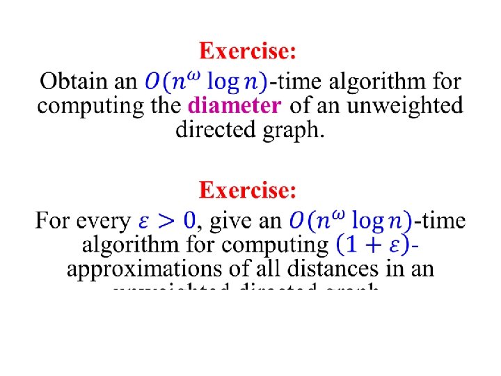
 algorithm for the directed unweighted APSP problem? An O(n")

 – add/remove an edge e • Vertex-Update(v) – add/remove")
 entries of the transitive closure matrix")

![Reachability via adjoint [Sankowski ’ 04] Let A be the symbolic adjacency matrix of](https://slidetodoc.com/presentation_image/2ead93bd2755be695e2ca87afd612657/image-137.jpg "Reachability via adjoint [Sankowski ’ 04] Let A be the symbolic adjacency matrix of")
 4 1 6 3 2 5 Is there a path")
 – add/remove an edge e • Vertex-Update(v) – add/remove")
![2 O(n ) update / O(1) query algorithm [Sankowski ’ 04] Let p n](https://slidetodoc.com/presentation_image/2ead93bd2755be695e2ca87afd612657/image-140.jpg "2 O(n ) update / O(1) query algorithm [Sankowski ’ 04] Let p n")

")
 Can be made worst-case")

 – add/remove an edge e • Vertex-Update(v) – add/remove")
![Finding triangles in O(m 2 /( +1)) time [Alon-Yuster-Z (1997)] Let be a parameter.](https://slidetodoc.com/presentation_image/2ead93bd2755be695e2ca87afd612657/image-146.jpg "Finding triangles in O(m 2 /( +1)) time [Alon-Yuster-Z (1997)] Let be a parameter.")
≠ 0 ?")
![Color coding [AYZ ’ 95] Assign each vertex v a random number c(v) from](https://slidetodoc.com/presentation_image/2ead93bd2755be695e2ca87afd612657/image-148.jpg "Color coding [AYZ ’ 95] Assign each vertex v a random number c(v) from")
- Slides: 148
Matrix Multiplication and Graph Algorithms Uri Zwick Tel Aviv University February 2015 Last updated: June 10, 2015
Short introduction to Fast matrix multiplication
Algebraic Matrix Multiplication j i = Can be computed naively in O(n 3) time.
Matrix multiplication algorithms Complexity Authors 3 n — n 2. 81 Strassen (1969) … 2. 38 n Coppersmith-Winograd (1990) 2+o(1) Conjecture/Open problem: n ? ? ?
Matrix multiplication algorithms - Recent developments Complexity Authors 2. 376 n Coppersmith-Winograd (1990) 2. 374 n Stothers (2010) 2. 3729 n Williams (2011) n 2. 37287 Le Gall (2014) Conjecture/Open problem: n 2+o(1) ? ? ?
Multiplying 2 2 matrices 8 multiplications 4 additions Works over any ring!
Multiplying n n matrices 8 multiplications 4 additions T(n) = 8 T(n/2) + O(n 2) T(n) = O(nlg 8)=O(n 3) ( lg n = log 2 n )
“Master method” for recurrences [CLRS 3 rd Ed. , p. 94]
Strassen’s 2 2 algorithm Subtraction! 7 multiplications 18 additions/subtractions Works over any ring! (Does not assume that multiplication is commutative)
Strassen’s n n algorithm View each n n matrix as a 2 2 matrix whose elements are n/2 matrices Apply the 2 2 algorithm recursively T(n) = 7 T(n/2) + O(n 2) T(n) = O(nlg 7)=O(n 2. 81) Exercise: If n is a power of 2, the algorithm uses nlg 7 multiplications and 6(nlg 7 n 2) additions/subtractions
Winograd’s 2 2 algorithm Works over any ring! 7 multiplications 15 additions/subtractions
Exponent of matrix multiplication Let be the “smallest” constant such that two n n matrices can be multiplies in O(n ) time 2 ≤ < 2. 37287 ( Many believe that =2+o(1) )
Inverses / Determinants The title of Strassen’s 1969 paper is: “Gaussian elimination is not optimal” Other matrix operations that can be performed in O(n ) time: • Computing inverses: A 1 • Computing determinants: det(A) • Solving systems of linear equations: Ax = b • Computing LUP decomposition: A = LUP • Computing characteristic polynomials: det(A− I) • Computing rank(A) and a corresponding submatrix
Block-wise Inversion Provided that A and S are invertible If M is (square, real, symmetric) positive definite, (M=NTN, N invertible), then M satisfies the conditions above If M is a real invertible square matrix, M 1=(MTM) 1 MT Over other fields, use LUP factorization
Positive Definite Matrices A real symmetric n n matrix A is said to be positive-definite (PD) iff x. TAx>0 for every x≠ 0 Theorem: (Cholesky decomposition) A is PD iff A=BTB where B invertible Exercise: If M is PD then the matrices A and S encountered in the inversion algorithm are also PD
LUP decomposition n m A n m = m L m n U n L is unit lower triangular U is upper triangular P is a permutation matrix Can be computed in O(n ) time P
LUP decomposition (in pictures) [Bunch-Hopcroft (1974)] n m A = [AHU’ 74, Section 6. 4 p. 234]
LUP decomposition (in pictures) [Bunch-Hopcroft (1974)] n m/2 B m/2 C n m =m L 1 I m U 1 D = CP 1− 1 Compute an LUP factorization of B [AHU’ 74, Section 6. 4 p. 234] n n P 1
LUP decomposition (in pictures) [Bunch-Hopcroft (1974)] n m/2 B m/2 C n m =m L 1 I m n E U 1 F D n P 1 Perform row operations to zero F n m = m L 1 FE− 1 I [AHU’ 74, Section 6. 4 p. 234] m n E U 1 G= D−FE− 1 U n 1 P 1
LUP decomposition (in pictures) [Bunch-Hopcroft (1974)] n n m m/2 U 1 m/2 G’ =m I L 2 m n H = U 1 P 3− 1 U 2 n Compute an LUP factorization of G’ m n m A =m L 1 FE− 1 L 2 [AHU’ 74, Section 6. 4 p. 234] m U 2 P 1 P 2 P 3 n n H I n P 3 P 1
LUP decomposition (in pictures) [Bunch-Hopcroft (1974)] Where did we use the permutations? In the base case m=1 !
LUP decomposition - Complexity [Bunch-Hopcroft (1974)]
Inversion Matrix Multiplication Exercise: Show that matrix multiplication and matrix squaring are essentially equivalent.
Checking Matrix Multiplication C = AB ?
Matrix Multiplication Determinants / Inverses Combinatorial applications? Transitive closure Shortest Paths Perfect/Maximum matchings Dynamic transitive closure and shortest paths k-vertex connectivity Counting spanning trees
BOOLEAN MATRIX MULTIPLICATION and TRANSIVE CLOSURE
Boolean Matrix Multiplication j i = Can be computed naively in O(n 3) time.
Algebraic Product O(n ) algebraic operations Boolean Product ? operations But, we can work Logical or ( ) over the integers! on O(log n)-bit words has no inverse! (modulo n+1) O(n )
Witnesses for Boolean Matrix Multiplication A matrix W is a matrix of witnesses iff Can we compute witnesses in O(n ) time?
Transitive Closure Let G=(V, E) be a directed graph. The transitive closure G*=(V, E*) is the graph in which (u, v) E* iff there is a path from u to v. Can be easily computed in O(mn) time. Can also be computed in O(n ) time.
Adjacency matrix of a directed graph 4 1 6 3 2 5 Exercise 0: If A is the adjacency matrix of a graph, then (Ak)ij=1 iff there is a path of length k from i to j.
Transitive Closure using matrix multiplication Let G=(V, E) be a directed graph. If A is the adjacency matrix of G, then (A I)n 1 is the adjacency matrix of G*. The matrix (A I)n 1 can be computed by log n squaring operations in O(n log n) time. It can also be computed in O(n ) time.
B A B C D A X = D C E F X* = (A BD*C)* EBD* D*CE D* GBD* = G H TC(n) ≤ 2 TC(n/2) + 6 BMM(n/2) + O(n 2)
Exercise 1: Give O(n ) algorithms for findning, in a directed graph, a) a triangle b) a simple quadrangle c) a simple cycle of length k. Hints: 1. In an acyclic graph all paths are simple. 2. In c) running time may be exponential in k. 3. Randomization makes solution much easier.
MIN-PLUS MATRIX MULTIPLICATION and ALL-PAIRS SHORTEST PATHS (APSP)
An interesting special case of the APSP problem A B 20 17 30 2 10 23 5 20 Min-Plus product
Min-Plus Products
Solving APSP by repeated squaring If W is an n by n matrix containing the edge weights of a graph. Then Wn is the distance matrix. By induction, Wk gives the distances realized by paths that use at most k edges. D W for i 1 to log 2 n do D D*D Thus: APSP(n) MPP(n) log n Actually: APSP(n) = O(MPP(n))
B A B C D A X = D C E F X* = (A BD*C)* EBD* D*CE D* GBD* = G H APSP(n) ≤ 2 APSP(n/2) + 6 MPP(n/2) + O(n 2)
Algebraic Product O(n ) Min-Plus Product ? min operation has no inverse! To be continued…
PERFECT MATCHINGS
Matchings A matching is a subset of edges that do not touch one another.
Matchings A matching is a subset of edges that do not touch one another.
Perfect Matchings A matching is perfect if there are no unmatched vertices
Perfect Matchings A matching is perfect if there are no unmatched vertices
Algorithms for finding perfect or maximum matchings Combinatorial approach: A matching M is a maximum matching iff it admits no augmenting paths
Algorithms for finding perfect or maximum matchings Combinatorial approach: A matching M is a maximum matching iff it admits no augmenting paths
Combinatorial algorithms for finding perfect or maximum matchings In bipartite graphs, augmenting paths, and hence maximum matchings, can be found quite easily using max flow techniques. In non-bipartite the problem is much harder. (Edmonds’ Blossom shrinking techniques) Fastest running time (in both cases): O(mn 1/2) [Hopcroft-Karp] [Micali-Vazirani]
Adjacency matrix of a undirected graph 4 1 6 3 2 5 The adjacency matrix of an undirected graph is symmetric.
Matchings, Permanents, Determinants Exercise: Show that if A is the adjacency matrix of a bipartite graph G, then per(A) is the number of perfect matchings in G. Unfortunately computing the permanent is #P-complete…
Tutte’s matrix (Skew-symmetric symbolic adjacency matrix) 4 1 2 6 3 5
Tutte’s theorem 1 2 4 3 There are perfect matchings
Tutte’s theorem 1 2 4 3 No perfect matchings
Proof of Tutte’s theorem Every permutation Sn defines a cycle collection 1 2 3 4 6 5 7 9 10 8
Cycle covers A permutation Sn for which {i, (i)} E, for 1 ≤ i ≤ n, defines a cycle cover of the graph. 1 2 3 4 6 5 7 9 8 Exercise: If ’ is obtained from by reversing the direction of a cycle, then sign( ’)=sign( ). Depending on the parity of the cycle!
Reversing Cycles 1 1 2 2 3 4 6 5 7 9 8 Depending on the parity of the cycle!
Proof of Tutte’s theorem (cont. ) The permutations Sn that contain an odd cycle cancel each other! We effectively sum only over even cycle covers. Different even cycle covers define different monomials, which do not cancel each other out. A graph contains a perfect matching iff it contains an even cycle cover.
Proof of Tutte’s theorem (cont. ) A graph contains a perfect matching iff it contains an even cycle cover. Perfect Matching Even cycle cover
Proof of Tutte’s theorem (cont. ) A graph contains a perfect matching iff it contains an even cycle cover. Even cycle cover Perfect matching
Pfaffians
An algorithm for perfect matchings? Problem: det(A) is a symbolic expression that may be of exponential size! Lovasz’s solution: Replace each variable xij by a random element of Zp, where p= (n 2) is a prime number
The Schwartz-Zippel lemma [Schwartz (1980)] [Zippel (1979)] Proof by induction on n. For n=1, follows from the fact that polynomial of degree d over a field has at most d roots
Proof of Schwartz-Zippel lemma Let k d be the largest i such that
Lovasz’s algorithm for existence of perfect matchings • Construct the Tutte matrix A. • Replace each variable xij by a random element of Zp, where p n 2 is prime. • Compute det(A). • If det(A) 0, say ‘yes’, otherwise ‘no’. If algorithm says ‘yes’, then the graph contains a perfect matching. If the graph contains a perfect matching, then the probability that the algorithm says ‘no’, is at most n/p 1/n.
Exercise: In the proof of Tutte’s theorem, we considered det(A) to be a polynomial over the integers. Is theorem true when we consider det(A) as a polynomial over Zp ?
Parallel algorithms PRAM – Parallel Random Access Machine NC - class of problems that can be solved in O(logkn) time, for some fixed k, using a polynomial number of processors NCk - class of problems that can be solved using uniform bounded fan-in Boolean circuits of depth O(logkn) and polynomial size
Parallel matching algorithms Determinants can be computed very quickly in parallel DET NC 2 Perfect matchings can be detected very quickly in parallel (using randomization) PERFECT-MATCH RNC 2 Open problem: ? ? ? PERFECT-MATCH NC ? ? ?
Finding perfect matchings Self Reducibility Delete an edge and check whethere is still a perfect matching Needs O(n 2) determinant computations Running time O(n +2) Fairly slow… Not parallelizable!
Finding perfect matchings Rabin-Vazirani (1986): An edge {i, j} E is contained in a perfect matching iff (A 1)ij 0. Leads immediately to an O(n +1) algorithm: Find an allowed edge {i, j} E , delete it and its vertices from the graph, and recompute A 1. Mucha-Sankowski (2004): Recomputing A 1 from scratch is very wasteful. Running time can be reduced to O(n ) ! Harvey (2006): A simpler O(n ) algorithm.
Adjoint and Cramer’s rule 1 A with the j-th row and i-th column deleted Cramer’s rule:
Finding perfect matchings Rabin-Vazirani (1986): An edge {i, j} E is contained in a perfect matching iff (A 1)ij 0. 1 Leads immediately to an O(n +1) algorithm: Find an allowed edge {i, j} E , delete it and its vertices from the graph, and recompute A 1. Still not parallelizable
Finding unique minimum weight perfect matchings [Mulmuley-Vazirani (1987)] Suppose that edge {i, j} E has integer weight wij Suppose that there is a unique minimum weight perfect matching M of total weight W Exercise: Prove the last two claims
Isolating lemma [Mulmuley-Vazirani (1987)] Suppose that G has a perfect matching Assign each edge {i, j} E a random integer weight wij [1, 2 m] Lemma: With probability of at least ½, the minimum weight perfect matching of G is unique Lemma holds for general collections of sets, not just perfect matchings
Proof of Isolating lemma [Mulmuley-Vazirani (1987)] An edge {i, j} is ambivalent if there is a minimum weight perfect matching that contains it and another that does not If minimum not unique, at least one edge is ambivalent Assign weights to all edges except {i, j} Let aij be the largest weight for which {i, j} participates in some minimum weight perfect matchings If wij<aij , then {i, j} participates in all minimum weight perfect matchings {i, j} can be ambivalent only if wij=aij The probability that {i, j} is ambivalent is at most 1/(2 m) !
Finding perfect matchings [Mulmuley-Vazirani (1987)] Choose random weights in [1, 2 m] Compute determinant and adjoint Read of a perfect matching (w. h. p. ) Is using 2 m-bit integers cheating? Not if we are willing to pay for it! Complexity is O(mn ) ≤ O(n +2) Finding perfect matchings in RNC 2 Improves an RNC 3 algorithm by [Karp-Upfal-Wigderson (1986)]
Multiplying two N-bit numbers “School method’’ [Schönhage-Strassen (1971)] [Fürer (2007)] [De-Kurur-Saha-Saptharishi (2008)] For our purposes…
Karatsuba’s Integer Multiplication [Karatsuba and Ofman (1962)] x = x 1 2 n/2 + x 0 y = y 1 2 n/2 + y 0 u = (x 1 + x 0)(y 1 + y 0) v = x 1 y 1 w = x 0 y 0 xy = v 2 n + (u−v−w)2 n/2 + w T(n) = 3 T(n/2+1)+O(n) T(n) = (nlg 3) = O(n 1. 59)
Finding perfect matchings The story not over yet… [Mucha-Sankowski (2004)] Recomputing A 1 from scratch is wasteful. Running time can be reduced to O(n ) ! [Harvey (2006)] A simpler O(n ) algorithm.
Sherman-Morrison formula Inverse of a rank one update is a rank one update of the inverse Inverse can be updated in O(n 2) time
Finding perfect matchings A simple O(n 3)-time algorithm [Mucha-Sankowski (2004)] Let A be a random Tutte matrix Compute A 1 Repeat n/2 times: Find an edge {i, j} that appears in a perfect matching (i. e. , Ai, j 0 and (A 1)i, j 0) Zero all entries in the i-th and j-th rows and columns of A, and let Ai, j=1, Aj, i= 1 Update A 1
Exercise: Is it enough that the random Tutte matrix A, chosen at the beginning of the algorithm, is invertible? What is the success probability of the algorithm if the elements of A are chosen from Zp
Sherman-Morrison-Woodbury formula Inverse of a rank k update is a rank k update of the inverse Can be computed in O(M(n, k, n)) time
A Corollary [Harvey (2009)]
Harvey’s algorithm [Harvey (2009)] Go over the edges one by one and delete an edge if there is still a perfect matching after its deletion Check the edges for deletion in a clever order! Concentrate on small portion of the matrix and update only this portion after each deletion Instead of selecting edges, as done by Rabin-Vazirani, we delete edges
Can we delete edge {i, j}? Set ai, j and aj, i to 0 Check whether the matrix is still invertible We are only changing AS, S , where S={i, j} New matrix is invertible iff {i, j} can be deleted iff ai, j bi, j 1 (mod p)
Harvey’s algorithm [Harvey (2009)] Find-Perfect-Matching(G=(V=[n], E)): Let A be a the Tutte matrix of G Assign random values to the variables of A If A is singular, return ‘no’ Compute B = A 1 Delete-In(V) Return the set of remaining edges
Harvey’s algorithm [Harvey (2009)] Before calling Delete-In(S) and Delete-Between(S, T) keep copies of A[S, S], B[S, S], A[S∪T, S∪T], B[S∪T, S∪T]
Delete-In(S): If |S| = 1 then return Divide S in half: S = S 1 ∪ S 2 For i ∈ {1, 2} Delete-In(Si) Update B[S, S] Delete-Between(S 1, S 2) Invariant: When entering and exiting, A is up to date, and B[S, S]=(A 1)[S, S]
Same Invariant Delete-Between(S, T): with B[S∪T, S∪T] If |S| = 1 then Let s ∈ S and t ∈ T If As, t = 0 and As, t Bs, t − 1 then // Edge {s, t} can be deleted Set As, t = At, s = 0 Update B [S∪T, S∪T] // (Not really necessary!) Else Divide in half: S = S 1 ∪ S 2 and T = T 1 ∪ T 2 For i ∈ {1, 2} and for j ∈ {1, 2} Delete-Between(Si, Tj ) Update B[S∪T, S∪T]
Maximum matchings Theorem: [Lovasz (1979)] Let A be the symbolic Tutte matrix of G. Then rank(A) is twice the size of the maximum matching in G. If |S|=rank(A) and A[S, *] is of full rank, then G[S] has a perfect matching, which is a maximum matching of G. Corollary: Maximum matchings can be found in O(n ) time
“Exact matchings” [MVV (1987)] Let G be a graph. Some of the edges are red. The rest are black. Let k be an integer. Is there a perfect matching in G with exactly k red edges? Exercise*: Give a randomized polynomial time algorithm for the exact matching problem No deterministic polynomial time algorithm is known for the exact matching problem!
MIN-PLUS MATRIX MULTIPLICATION and ALL-PAIRS SHORTEST PATHS (APSP)
Fredman’s trick [Fredman (1976)] The min-plus product of two n n matrices can be deduced after only O(n 2. 5) additions and comparisons. It is not known how to implement the algorithm in O(n 2. 5) time.
Algebraic Decision Trees a 17 a 19 ≤ b 92 b 72 no yes … c 11=a 17+b 71 c 12=a 14+b 42 c 11=a 13+b 31 c 12=a 15+b 52 . . . … c 11=a 18+b 81 c 12=a 16+b 62 c 11=a 12+b 21 c 12=a 13+b 32 . . .
Breaking a square product into several rectangular products m B 1 n A 1 A 2 B 2 MPP(n) ≤ (n/m) (MPP(n, m, n) + n 2)
Fredman’s trick m [Fredman (1976)] n ai, r+br, j ≤ ai, s+bs, j A B m n ai, r ai, s ≤ bs, j br, j Naïve calculation requires n 2 m operations Fredman observed that the result can be inferred after performing only O(nm 2) operations
Fredman’s trick (cont. ) ai, r+br, j ≤ ai, s+bs, j ai, r ai, s ≤ bs, j br, j The ordering of the elements in the sorted list determines the result of the min-plus product !!!
Sorting differences ai, r+br, j ≤ ai, s+bs, j ai, r ai, s ≤ bs, j br, j
All-Pairs Shortest Paths in directed graphs with “real” edge weights Running time Authors [Floyd (1962)] [Warshall (1962)] [Fredman (1976)] [Williams (2014)]
• Computing a min-plus product • APSP in weighted directed graphs • APSP in weighted undirected graphs • Finding a negative triangle • Finding a minimum weight cycle (non-negative edge weights) • Verifying a min-plus product • Finding replacement paths
UNWEIGHTED UNDIRECTED SHORTEST PATHS
2 Distances in G and its square G Let G=(V, E). Then G 2=(V, E 2), where (u, v) E 2 if and only if (u, v) E or there exists w V such that (u, w), (w, v) E Let δ (u, v) be the distance from u to v in G. Let δ 2(u, v) be the distance from u to v in G 2.
Distances in G and its square G 2 (cont. ) Lemma: δ 2(u, v) = δ(u, v)/2 , for every u, v V. δ 2(u, v) ≤ δ(u, v)/2 δ(u, v) ≤ 2δ 2(u, v) Thus: δ(u, v) = 2δ 2(u, v) or δ(u, v) = 2δ 2(u, v) 1
Even distances Lemma: If δ(u, v) = 2δ 2(u, v) then for every neighbor w of v we have δ 2(u, w) ≥ δ 2(u, v). Let A be the adjacency matrix of the G. Let C be the distance matrix of G 2
Odd distances Lemma: If δ(u, v) = 2δ 2(u, v)– 1 then for every neighbor w of v we have δ 2(u, w) δ 2(u, v) and for at least one neighbor δ 2(u, w) < δ 2(u, v). Exercise: Prove the lemma. Let A be the adjacency matrix of the G. Let C be the distance matrix of G 2
Assume that A has Seidel’s algorithm [Seidel (1995)] 1’s on the diagonal. 1. If A is an all one matrix, then all distances are 1. 2. Compute A 2, the adjacency matrix of the squared graph. 3. Find, recursively, the distances in the squared graph. 4. Decide, using one integer matrix multiplication, for every two vertices u, v, whether their distance is twice the distance in the square, or twice minus 1. Algorithm APD(A) Boolean matrix if A=J then multiplicaion return J–I else C←APD(A 2) X←CA , deg←Ae dij← 2 cij– [xij< cijdegj] Integer matrix return D multiplicaion end Complexity: O(n log n)
Exercise+: Obtain a version of Seidel’s algorithm that uses only Boolean matrix multiplications. Hint: Look at distances also modulo 3.
Distances vs. Shortest Paths We described an algorithm for computing all distances. How do we get a representation of the shortest paths? We need witnesses for the Boolean matrix multiplication.
Witnesses for Boolean Matrix Multiplication A matrix W is a matrix of witnesses iff Can be computed naively in O(n 3) time. Can also be computed in O(n log n) time.
Exercise n+1: a) Obtain a deterministic O(n )-time algorithm for finding unique witnesses. b) Let 1 ≤ d ≤ n be an integer. Obtain a randomized O(n )-time algorithm for finding witnesses for all positions that have between d and 2 d witnesses. c) Obtain an O(n log n)-time randomized algorithm for finding all witnesses. Hint: In b) use sampling.
All-Pairs Shortest Paths in graphs with small integer weights Undirected graphs. Edge weights in {0, 1, …M} Running time Authors Mn [Shoshan-Zwick ’ 99] Improves results of [Alon-Galil-Margalit ’ 91] [Seidel ’ 95]
DIRECTED SHORTEST PATHS
Using matrix multiplication to compute min-plus products
Using matrix multiplication to compute min-plus products Assume: 0 ≤ aij , bij ≤ M n polynomial products Mn M operations per polynomial product = operations per min-plus product
Trying to implement the repeated squaring algorithm D W for i 1 to log 2 n D D*D Consider an easy case: all weights are 1 After the i-th iteration, the finite elements in D are in the range {1, …, 2 i}. The cost of the min-plus product is 2 i n The cost of the last product is n +1 !!!
Sampled Repeated Squaring [Z (1998)] The is also a slightly more complicated With high probability, deterministic algorithm all distances are correct!
Sampled Distance Products (Z ’ 98) The matrices get smaller and smaller but the elements get larger and larger
Sampled Repeated Squaring - Correctness D W for i 1 to log 3/2 n do { s (3/2)i+1 B rand(V, (9 n ln n)/s) D min{ D , D[V, B]*D[B, V] } } Invariant: After the i-th iteration, distances that are attained using at most (3/2)i edges are correct. Consider a shortest path that uses at most (3/2)i+1 edges at most Let s = (3/2)i+1 at most Failure probability :
Rectangular Matrix multiplication p n n n p = n Naïve complexity: n 2 p [Coppersmith (1997)] [Huang-Pan (1998)] n 1. 85 p 0. 54+n 2+o(1) For p ≤ n 0. 29, complexity = n 2+o(1) !!!
Rectangular Matrix multiplication n 0. 29 n = n [Coppersmith (1997)] n n 0. 29 by n 0. 29 n 2+o(1) n operations! = 0. 29…
Rectangular Matrix multiplication p n n n p = n [Huang-Pan (1998)] Break into q q and q q sub-matrices
Complexity of APSP algorithm The i-th iteration: n/s s = (3/2)i+1 n “Fast” matrix multiplication n /s n Naïve matrix multiplication The elements are of absolute value at most Ms
Complexity of APSP algorithm
Open problem: Can APSP in unweighted directed graphs be solved in O(n ) time? [Yuster-Z (2005)] A directed graphs can be processed in O(n ) time so that any distance query can be answered in O(n) time. Corollary: SSSP in directed graphs in O(n ) time. Also obtained, using a different technique, by [Sankowski (2005)]
The preprocessing algorithm [YZ (2005)]
Twice Sampled Distance Products
The query answering algorithm v u
The preprocessing algorithm: Correctness at most
Answering distance queries Directed graphs. Edge weights in {−M, …, 0, …M} Preprocessing time Query time Authors [Yuster-Zwick n (2005)] In particular, any Mn 1. 38 distances can be computed in Mn 2. 38 time. Mn 2. 38 For dense enough graphs with small enough edge weights, this improves on Goldberg’s SSSP algorithm. Mn 2. 38 vs. mn 0. 5 log M
Approximate All-Pairs Shortest Paths in graphs with non-negative integer weights (1+ε)-approximate distances Running time Authors (n 2. 38 log M)/ε [Z (1998)]
Open problems An O(n ) algorithm for the directed unweighted APSP problem? An O(n 3 ε) algorithm for the APSP problem with edge weights in {1, 2, …, n}? An O(n 2. 5 ε) algorithm for the SSSP problem with edge weights in { 1, 0, 1, 2, …, n}?
DYNAMIC TRANSITIVE CLOSURE
Dynamic transitive closure • Edge-Update(e) – add/remove an edge e • Vertex-Update(v) – add/remove edges touching v. • Query(u, v) – is there are directed path from u to v? [Sankowski ’ 04] Edge-Update n 2 n 1. 575 n 1. 495 Vertex-Update n 2 – – Query 1 n 0. 575 n 1. 495 (improving [Demetrescu-Italiano ’ 00], [Roditty ’ 03])
Inserting/Deleting and edge May change (n 2) entries of the transitive closure matrix
Symbolic Adjacency matrix 4 1 6 3 2 5
Reachability via adjoint [Sankowski ’ 04] Let A be the symbolic adjacency matrix of G. (With 1 s on the diagonal. ) There is a directed path from i to j in G iff
Reachability via adjoint (example) 4 1 6 3 2 5 Is there a path from 1 to 5?
Dynamic transitive closure • Edge-Update(e) – add/remove an edge e • Vertex-Update(v) – add/remove edges touching v. • Query(u, v) – is there are directed path from u to v? Dynamic matrix inverse • Entry-Update(i, j, x) – Add x to Aij • Row-Update(i, v) – Add v to the i-th row of A • Column-Update(j, u) – Add u to the j-th column of A • Query(i, j) – return (A-1)ij
2 O(n ) update / O(1) query algorithm [Sankowski ’ 04] Let p n 3 be a prime number Assign random values aij 2 Fp to the variables xij 1 Maintain A over Fp Edge-Update Entry-Update Vertex-Update Row-Update + Column-Update Perform updates using the Sherman-Morrison formula Small error probability (by the Schwartz-Zippel lemma)
Lazy updates Consider single entry updates
Lazy updates (cont. )
Lazy updates (cont. ) Can be made worst-case
Even Lazier updates
Dynamic transitive closure • Edge-Update(e) – add/remove an edge e • Vertex-Update(v) – add/remove edges touching v. • Query(u, v) – is there are directed path from u to v? [Sankowski ’ 04] Edge-Update n 2 n 1. 575 n 1. 495 Vertex-Update n 2 – – Query 1 n 0. 575 n 1. 495 (improving [Demetrescu-Italiano ’ 00], [Roditty ’ 03])
Finding triangles in O(m 2 /( +1)) time [Alon-Yuster-Z (1997)] Let be a parameter. . = m( -1) /( +1) High degree vertices: vertices of degree . Low degree vertices: vertices of degree < . There at most 2 m/ high degree vertices = 163
Finding longer simple cycles A graph G contains a Ck iff Tr(Ak)≠ 0 ? We want simple cycles! 164
Color coding [AYZ ’ 95] Assign each vertex v a random number c(v) from {0, 1, . . . , k 1}. Remove all edges (u, v) for which c(v)≠c(u)+1 (mod k). All cycles of length k in the graph are now simple. If a graph contains a Ck then with a probability of at least k k it still contains a Ck after this process. An improved version works with probability 2 O(k). Can be derandomized at a logarithmic cost. 165